Building an Assessment Pipeline with mirtverse: Automation with Human Oversight

Developing a test involves many psychometric steps, from writing a blueprint to monitoring an item bank, and each step involves decisions that should be checked and documented. In this post, I explain why we need assessment pipelines that automate routine psychometric checks while keeping humans in charge of the decisions. Then, I introduce the assessment pipeline in the mirtverse package and take a certification exam through its stages, from the blueprint to bank monitoring.

(17 min read)

Image generated by ChatGPT

Introduction

In my previous post, I introduced mirtverse (Bulut, 2026), an R package that makes the mirt package (Chalmers, 2012) easier to use for everyday item response theory (IRT) analyses. In this post, I want to focus on a bigger question: How do we organize all the psychometric work that goes into a test, from the moment we decide what the test should measure to the moment we retire its items?

A test passes through many hands before a score reaches a test taker. Someone writes a blueprint, item writers draft the items, content and sensitivity reviewers check them, psychometricians plan a field test, calibrate the items, check for bias, link the new items to an item bank, assemble the forms, help a panel set cut scores, and so on. Each of these steps produces numbers, and each set of numbers leads to a decision: Is this item miskeyed? Is this DIF large enough to remove the item? Is the reliability high enough for a pass/fail decision? These steps are described in detail in the testing literature (Downing, 2006; Lane et al., 2016), and the Standards for Educational and Psychological Testing (American Educational Research Association et al., 2014) expect testing programs to document the evidence and the decisions behind their scores.

In practice, however, these steps are often scattered across different scripts, different software, and different people’s inboxes. A DIF result lives in one spreadsheet, the decision about it lives in an email thread, and the R code that produced it may or may not be the version that was actually run. When a problem surfaces months later, it can be very difficult to reconstruct what was checked, what was found, and who decided what. In this post, I argue that we need assessment pipelines that automate the routine checks while keeping humans in charge of the decisions, and I show how the assessment pipeline in mirtverse does this.

Why Do We Need Assessment Pipelines?

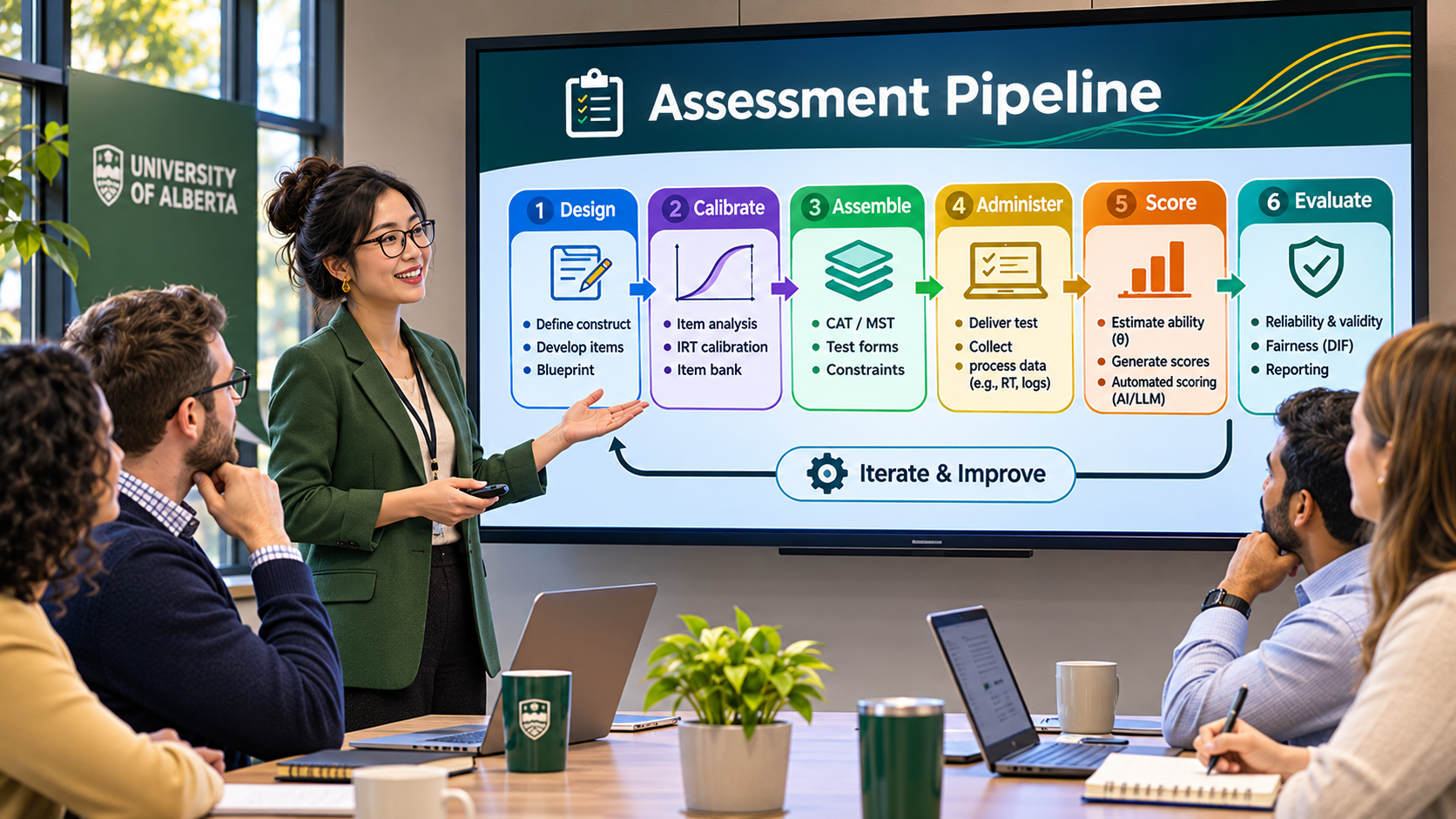
The word “pipeline” comes from software engineering and data science, where it refers to a sequence of steps that turns raw input into a finished product, with each step feeding the next. An assessment pipeline applies the same idea to test development: response data (and items, blueprints, and reviews) go in, and calibrated items, assembled forms, cut scores, scores, and a technical report come out.

Automating these steps has clear benefits:

• Consistency: The same checks are applied in the same way every time, regardless of who runs the analysis or how busy they are.
• Completeness: Nothing is skipped by accident. If the pipeline checks local dependence after every calibration, it is checked after every calibration.
• Reproducibility: Every step is recorded as code, so the whole analysis can be rerun and audited.
• Speed: Routine checks that used to take days can be done in minutes, which leaves more time for the decisions that really need expert judgment.

But full automation is not what we want either. Psychometric decisions are rarely mechanical. An item with large DIF may be removed, revised, or kept after a content review shows that the difference reflects the construct rather than bias. A reliability of .83 may be acceptable for a low-stakes diagnostic test but not for a certification exam. A miskey flag may point to a wrong key, or to a correct but very difficult item. These decisions depend on the purpose of the test, the intended use of the scores, and evidence that is not in the response data (Kane, 2013). They should be made by people who are accountable for them.

This is where the idea of human-in-the-loop systems comes in (Amershi et al., 2014). In a human-in-the-loop pipeline, the machine does what it does well (running checks, comparing statistics with thresholds, keeping records), and humans do what they do well (interpreting the evidence in context and making decisions). The key design question is how the two interact. In my view, a good assessment pipeline should have four properties:

1. Checks after every stage. Each stage should end with a set of checks (I call them gates) that compare the results with explicit, changeable thresholds.
2. Graded flags. Not every finding is equally serious. Some are for awareness, some need a psychometrician’s review, and some make later stages unsafe.
3. Recorded decisions. When a human accepts, overrides, or fixes a flag, the decision and its reason should be recorded next to the evidence.
4. An option to stop. For high-stakes programs, the pipeline should be able to refuse to continue while serious flags are still open.

The Assessment Pipeline in mirtverse

mirtverse (version 0.2.0) implements this idea in a single R object created with mv_pipeline(). The pipeline has 13 stages, numbered from 0 to 12, that follow a test from its blueprint to the monitoring of its item bank. The following figure shows the stages and the functions that run them.

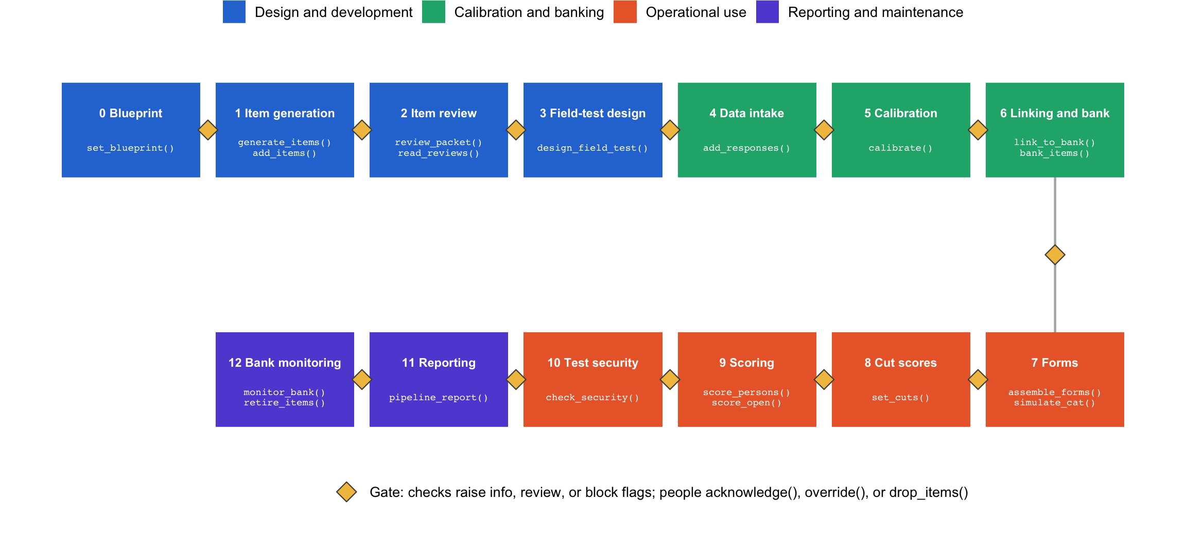
Figure 1: The 13 stages of the mirtverse assessment pipeline. Each stage ends with a gate (diamond) that raises flags for human review.

Each stage does its work and then runs its gate. The gate compares the results with thresholds and records what it finds as flags. Flags come in three levels:

• info: for awareness only.
• review: something a psychometrician should look at.
• block: a problem that makes later stages unsafe.

People respond to the flags with three functions. acknowledge() accepts a flag (with an optional note), override() keeps going despite a block flag (and requires a written reason), and drop_items() removes the items behind a flag, which marks the flag as fixed. Every decision is logged, and the final report prints every flag next to the decision that was made about it.

By default, flags only warn, so all stages still run. This is useful for exploring the data or for pilot studies. With mv_pipeline(strict = TRUE), the pipeline becomes a real gatekeeper: a stage refuses to start while an earlier stage has open review or block flags. This guarantees that no problem can be passed over without a recorded human decision.

Example

Data

For this example, I use the certexam data set that comes with mirtverse. It contains the raw (unscored) answers of 1,200 candidates to a 32-item multiple-choice certification exam. Each candidate took the exam in English or French. The answer key is stored in certexam_key. The data are simulated, and they have several problems planted in them (as we will see, the gates find them).

dim(certexam)

[1] 1200   34

head(certexam[, 1:8])

     id language Q01 Q02 Q03 Q04 Q05 Q06
1 C0001   French   E   B   C   B   C   A
2 C0002  English   E   B   A   D   C   B
3 C0003  English   B   C   E   D   C   D
4 C0004  English   C   C   E   C   C   D
5 C0005  English   A   B   A   B   C   D
6 C0006   French   B   C   E   E   C   E

table(certexam$language)

English  French 
    750     450 

Starting the Pipeline

We start the pipeline with mv_pipeline(). Because this is a certification exam, I use the strict mode. I also set verbose = FALSE to keep the output short.

p <- mv_pipeline("Certification exam", strict = TRUE, verbose = FALSE)
p

<mv_pipeline> Certification exam
strict: open review and block flags stop the next stage; rules: standards

[ ] 0  Blueprint         not run
[ ] 1  Item generation   not run
[ ] 2  Item review       not run
[ ] 3  Field-test design not run
[ ] 4  Data intake       not run
[ ] 5  Calibration       not run
[ ] 6  Linking and bank  not run
[ ] 7  Forms             not run
[ ] 8  Cut scores        not run
[ ] 9  Scoring           not run
[ ] 10 Test security     not run
[ ] 11 Reporting         not run
[ ] 12 Bank monitoring   not run

No open flags.

Printing the pipeline shows the 13 stages and their status. All the thresholds used by the gates are stored in mv_rules(). The defaults follow common operational practice, and each one can be changed by name. For example, mv_rules(q3 = 0.25) relaxes the local dependence threshold, and mv_rules(preset = "lenient") relaxes all of them at once for a pilot study.

rules <- mv_rules()
length(rules)

[1] 71

rules[c("miskey_p", "q3", "reliability", "cut_accuracy", "cut_sem")]

$miskey_p
[1] 0.1

$q3
[1] 0.2

$reliability
[1] 0.8

$cut_accuracy
[1] 0.85

$cut_sem
[1] 0.35

Stage 0: The Blueprint

The blueprint is the contract that every later stage checks against. It defines what the test measures (i.e., the construct), how the scores will be used, and how many items each content area needs on a form. Our exam covers three content areas: Ethics (4 items per form), Practice (5 items), and Law (3 items). Since the scores will be used for a pass/fail decision, I also ask for a reliability of at least .85.

p <- set_blueprint(p, c(Ethics = 4, Practice = 5, Law = 3),
                   construct = "Professional knowledge for certification",
                   use = "pass/fail certification", reliability = 0.85)
p$blueprint$cells

# A tibble: 3 × 4
  cell     content  cognitive     n
  <chr>    <chr>    <chr>     <dbl>
1 Ethics   Ethics   <NA>          4
2 Practice Practice <NA>          5
3 Law      Law      <NA>          3

The reliability target I set here replaces the default reliability rule, so the calibration stage will hold the test to this standard.

Stages 1 and 2: Writing and Reviewing Items

The certexam items already exist, so these two stages do not apply to our main example. But they are a good place to see the human-in-the-loop idea at work, so let’s look at them with a small, separate pipeline.

Items can enter the pipeline in two ways. generate_items() drafts multiple-choice items (with keys and a rationale for every option) and open-ended items (with rubrics and anchor responses) for each blueprint cell using a large language model through the ellmer package. A second, independent model call then answers each item without seeing the key, and the gate flags disputed keys, weak distractors, near-duplicate items, and thin coverage of the blueprint. Items written by people enter the pipeline with add_items() and go through the same checks. Generated items are always treated as drafts: they need human review before they can be field-tested, and every item records its source (human or model).

# Needs an API key for the model provider (see mv_ask_setup())
p <- generate_items(p, n = 3)

For this example, I add four items written by people:

new_items <- data.frame(
  id   = c("ETH01", "ETH02", "PRA01", "LAW01"),
  cell = c("Ethics", "Ethics", "Practice", "Law"),
  stem = c("A client offers you a gift worth $500 after a successful case. What should you do first?",
           "A colleague asks you to sign a report you did not review. What is the most appropriate response?",
           "Which step should come first when a new client file is opened?",
           "Under the professional code, how long must client records be kept after a file is closed?"),
  A = c("Accept it and record it", "Sign it to save time", "Send an invoice", "1 year"),
  B = c("Decline and consult the gift policy", "Refuse and ask to review it first",
        "Run a conflict-of-interest check", "3 years"),
  C = c("Accept it privately", "Ask another colleague to sign", "Archive old files", "7 years"),
  D = c("Give it to a colleague", "Sign with a note", "Call the client", "Forever"),
  key = c("B", "B", "B", "C"))

p_items <- mv_pipeline("Item review example", verbose = FALSE)
p_items <- add_items(p_items, new_items)

Next, review_packet() writes a review form as a CSV file (which opens in Excel) with one row per item and reviewer. Each reviewer records a decision (accept, revise, or reject), whether the item measures its blueprint cell, and whether it raises any sensitivity concern. With ai_screen = TRUE, a language model first screens each item for possible bias and accessibility problems and adds its notes to the form, but the decisions remain with the human reviewers.

review_file <- tempfile(fileext = ".csv")
p_items <- review_packet(p_items, review_file, reviewers = c("Ana", "Ben", "Chen"))

reviews <- read.csv(review_file)
names(reviews)

 [1] "id"          "cell"        "type"        "item"       
 [5] "key"         "rubric"      "source"      "ai_screen"  
 [9] "reviewer"    "decision"    "aligned"     "sensitivity"
[13] "comment"    

In real life, the reviewers would fill in this form and send it back. Here, I fill it in myself to create a few typical situations: all reviewers accept most items, but two reviewers ask for a revision of ETH02, one reviewer thinks PRA01 does not measure its cell, one reviewer raises a sensitivity concern about ETH01, and only one reviewer has reviewed LAW01 so far.

reviews <- reviews %>%
  mutate(decision = "accept", aligned = "yes", sensitivity = "no", comment = "",
         decision = ifelse(id == "ETH02" & reviewer %in% c("Ben", "Chen"), "revise", decision),
         comment = ifelse(id == "ETH02", "Option D is also defensible", comment),
         aligned = ifelse(id == "PRA01" & reviewer == "Ana", "no", aligned),
         sensitivity = ifelse(id == "ETH01" & reviewer == "Chen", "yes", sensitivity)) %>%
  filter(!(id == "LAW01" & reviewer != "Ana"))

p_items <- read_reviews(p_items, reviews)
p_items$items %>% select(id, cell, source, status)

# A tibble: 4 × 4
  id    cell     source status  
  <chr> <chr>    <chr>  <chr>   
1 ETH01 Ethics   human  approved
2 ETH02 Ethics   human  revise  
3 PRA01 Practice human  approved
4 LAW01 Law      human  approved

read_reviews() sets each item’s status by majority vote: ETH02 goes back for revision, and the others are approved. But the gate also tells us why we should not simply move on:

flags(p_items) %>% select(check, target, value, level)

# A tibble: 5 × 4
  check              target    value                          level 
  <chr>              <chr>     <chr>                          <chr> 
1 under_reviewed     LAW01     1 reviewer(s)                  block 
2 alignment          PRA01     1 reviewer(s) disagree         review
3 sensitivity        ETH01     1 reviewer(s) raised a concern review
4 needs_revision     ETH02     reviewers asked for revision   review
5 reviewer_agreement reviewers Fleiss' kappa = 0.36           info  

LAW01 is approved, but only one person has reviewed it, which is a block flag. The other flags point to the concerns raised by individual reviewers, which would be easy to lose in a majority vote. Finally, the reviewers’ agreement is low (Fleiss’ kappa = .36), which suggests a calibration session before the next round of reviews. This is exactly the type of information that a review coordinator needs, and it comes with the record of who said what.

Stage 3: Field-Test Design

Now, back to our main pipeline. Before collecting calibration data, design_field_test() plans the field test: how many forms, which anchor items they share, and how many candidates each form needs. It then simulates how well the item parameters can be recovered under that plan.

p <- design_field_test(p, n_forms = 2, n_per_form = 600, items = 32,
                       reps = 2, seed = 1)
p$field_test$recovery

# A tibble: 1 × 4
   reps rmse_a rmse_d converged
  <dbl>  <dbl>  <dbl>     <dbl>
1     2  0.220  0.121         1

flags(p, stage = "field_test") %>% select(check, value, rule, level)

# A tibble: 1 × 4
  check    value                 rule        level 
  <chr>    <chr>                 <chr>       <chr> 
1 recovery RMSE of slopes = 0.22 RMSE <= 0.2 review

With two forms of 600 candidates, the discrimination parameters would be recovered with an RMSE of .22, which is slightly above the target of .20. The usual answer is more candidates per form. Let’s assume that the sample size is fixed by the testing window, so we accept the plan and record why:

p <- acknowledge(p, check = "recovery", note = "Sample fixed by the testing window")

Stage 4: Data Intake

add_responses() scores the raw answers with the key and then checks the data for missing responses, possible miskeys, straight-lining, rapid guessing, and sparse score categories. The group argument tells the pipeline which variable to use for the DIF analyses later.

p <- add_responses(p, certexam, items = 3:34, key = certexam_key,
                   id = "id", group = "language")
flags(p, stage = "intake") %>% select(check, target, value, rule, level)

# A tibble: 1 × 5
  check           target value                         
  <chr>           <chr>  <chr>                         
1 possible_miskey Q14    p = 0.18, item-total r = -0.23
  rule                        level
  <chr>                       <chr>
1 p < 0.1 or item-total r < 0 block

Item Q14 was answered correctly by only 18% of the candidates, and its item-total correlation is negative (-.23). In other words, the candidates who did well on the rest of the test were less likely to get Q14 right. This is the classic signature of a miskeyed item, and the gate raises a block flag. Now, let’s see what happens if we ignore it and try to calibrate the items:

p <- calibrate(p, model = "2PL")

Error:
! Calibration cannot start: 1 block flag(s) from earlier stages are still open.
  #2 [block] possible_miskey: Q14 (p = 0.18, item-total r = -0.23)
Fix them (for example with drop_items()), record a decision with acknowledge() (review flags) or override() (block flags), or use strict = FALSE.

Because we are in strict mode, the pipeline refuses to calibrate and tells us what we can do. Suppose the item writer confirms that the key was wrong. We remove the item, which marks the flag as fixed:

p <- drop_items(p, "Q14", note = "Key confirmed wrong by the item writer")

Stage 5: Calibration

Now the calibration can run. calibrate() fits the model with mirt and then checks convergence, model fit, local dependence, item fit, parameter ranges, DIF between the language groups, reliability, and person fit.

p <- calibrate(p, model = "2PL")
flags(p, stage = "calibration") %>% select(check, target, value, rule, level)

# A tibble: 5 × 5
  check            target        
  <chr>            <chr>         
1 dif_large        Q09           
2 local_dependence Q21 & Q22     
3 dif_moderate     Q27           
4 low_reliability  test          
5 person_misfit    22 respondents
  value                                                 rule     level
  <chr>                                                 <chr>    <chr>
1 MH D-DIF = -2.01, French vs English (favours English) ETS cat… block
2 Q3 = 0.27                                             |Q3| > … revi…
3 MH D-DIF = -1.01, French vs English (favours English) ETS cat… revi…
4 marginal reliability = 0.83                           reliabi… revi…
5 1.8% of respondents                                   Zh < -1… info 

The gate found three planted problems and one shortfall:

• Q09 has large DIF. Its Mantel-Haenszel D-DIF (Holland & Thayer, 1988) is -2.01, which falls into the ETS category C (large DIF) and favors the English-speaking candidates. This is a block flag.
• Q27 has moderate DIF (ETS category B), also favoring the English group.
• Q21 and Q22 are locally dependent (\(Q_3\) = .27; Yen (1984)). This often happens when two items share the same case or stimulus.
• The marginal reliability (.83) is below the .85 target that we set in the blueprint.

The person misfit flag is only for awareness: 1.8% of the candidates have unusual response patterns, which is about what we would expect by chance. None of these findings has an automatic answer. Each one requires a decision from someone who knows the exam:

p <- acknowledge(p, check = "local_dependence",
                 note = "Q21 and Q22 share a case; keep them apart on forms")
p <- override(p, check = "dif_large",
              note = "Translation reviewed; French version revised")
p <- acknowledge(p, check = "dif_moderate", note = "Sent to the bias panel")
p <- acknowledge(p, check = "low_reliability",
                 note = "Operational forms will be longer than the field test")

Note that override() is used for the block flag and it requires a written reason. These notes are not just comments in a script. They are stored in the pipeline object, attached to the flags they respond to, and printed in the final report.

Stage 6: The Item Bank

bank_items() stores the calibrated items in an item bank. In a later administration, link_to_bank() would put a new calibration on the bank’s scale through anchor items (with the Stocking-Lord, Haebara, mean-sigma, mean-mean, or fixed-anchor methods) and check the anchors for drift.

p <- bank_items(p, name = "Certification bank")
p$bank

<mv_bank> Certification bank: 31 items (31 active)
Item types: 2PL 31 
Location (b) from -2.37 to 3.05; median discrimination 0.90
Sources: Certification exam 

Stage 7: Test Forms

assemble_forms() builds parallel fixed forms with automated test assembly (Linden, 2005), using the eatATA package. Here, I ask for two 12-item forms that meet the content blueprint, maximize information at three ability levels (\(\theta\) = -1, 0, and 1), and keep the locally dependent items Q21 and Q22 apart (they are declared as enemy items). Adaptive and multistage designs are also available with simulate_cat() and assemble_mst(), which use the mirtCAT package.

content <- setNames(rep(c("Ethics", "Practice", "Law"), c(10, 12, 10)),
                    sprintf("Q%02d", 1:32))

p <- assemble_forms(p, length = 12, n_forms = 2, theta = c(-1, 0, 1),
                    content = content[names(content) != "Q14"],
                    blueprint = c(Ethics = 4, Practice = 5, Law = 3),
                    enemies = list(c("Q21", "Q22")))
p$forms$info

# A tibble: 6 × 4
   form theta information   sem
  <int> <dbl>       <dbl> <dbl>
1     1    -1        2.76 0.602
2     1     0        2.58 0.623
3     1     1        1.82 0.742
4     2    -1        2.62 0.617
5     2     0        2.67 0.612
6     2     1        1.86 0.734

The two forms meet the blueprint, keep Q21 and Q22 apart, and are parallel (their information differs by less than 10% at each ability level). However, the gate also checks measurement precision, and 12 items cannot reach a standard error of measurement (SEM) of .35 at any of these ability levels:

flags(p, stage = "forms") %>% select(check, target, value, rule)

# A tibble: 6 × 4
  check          target               value      rule       
  <chr>          <chr>                <chr>      <chr>      
1 form_precision form 1 at theta = -1 SEM = 0.60 SEM <= 0.35
2 form_precision form 1 at theta = 0  SEM = 0.62 SEM <= 0.35
3 form_precision form 1 at theta = 1  SEM = 0.74 SEM <= 0.35
4 form_precision form 2 at theta = -1 SEM = 0.62 SEM <= 0.35
5 form_precision form 2 at theta = 0  SEM = 0.61 SEM <= 0.35
6 form_precision form 2 at theta = 1  SEM = 0.73 SEM <= 0.35

For a pass/fail exam, what matters most is the precision near the cut score, which the next stage checks. So, we acknowledge these flags and move on:

p <- acknowledge(p, check = "form_precision",
                 note = "Precision near the cut matters most; checked at the cut-score stage")

Stage 8: Cut Scores

set_cuts() takes cut scores on the ability scale or the raw-score scale (or the ratings of a standard-setting panel) and estimates the classification accuracy and consistency of the pass/fail decisions (Lee, 2010). Let’s set the passing score to 18 out of 31.

p <- set_cuts(p, cuts = 18, scale = "raw", labels = c("Fail", "Pass"))
p$cuts$by_cut

# A tibble: 1 × 7
    cut label accuracy consistency kappa false_positive false_negative
  <int> <chr>    <dbl>       <dbl> <dbl>          <dbl>          <dbl>
1     1 Pass     0.861       0.809 0.613         0.0949         0.0445

flags(p, stage = "cuts") %>% select(check, target, value, rule)

# A tibble: 1 × 4
  check         target       value                      rule       
  <chr>         <chr>        <chr>                      <chr>      
1 cut_precision cut 1 (Pass) SEM = 0.42 at theta = 0.16 SEM <= 0.35

About 86% of the candidates are expected to be classified correctly, and 81% would receive the same decision if they took the exam again. Both values meet the default thresholds (.85 and .80). However, the standard error at the cut (which corresponds to \(\theta\) = 0.16) is .42, which is above the target of .35. The following figure shows why. It plots the standard error of the calibrated test across the ability scale, together with the location of the cut score.

theta <- seq(-3, 3, by = 0.05)
sem <- data.frame(theta = theta,
                  se = 1 / sqrt(testinfo(p$model, matrix(theta))))

ggplot(sem, aes(x = theta, y = se)) +
  geom_line(linewidth = 1.1, color = "#2a78d6") +
  geom_hline(yintercept = 0.35, linetype = "dotted", color = "grey40") +
  geom_vline(xintercept = 0.16, linetype = "dashed", color = "#eb6834") +
  annotate("text", x = 0.25, y = 0.95, label = "Cut score (raw = 18)",
           hjust = 0, color = "#eb6834") +
  annotate("text", x = -3, y = 0.37, label = "SEM target = .35",
           hjust = 0, vjust = 0, color = "grey40") +
  scale_y_continuous(limits = c(0, 1)) +
  labs(x = expression(theta), y = "Standard error of measurement") +
  theme_blog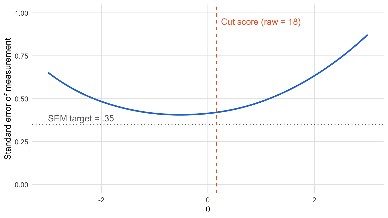

Figure 2: Standard error of measurement across the ability scale. The dashed line shows the cut score and the dotted line shows the SEM target.

The SEM curve never goes below .35. Even at its lowest point (around \(\theta\) = -0.5), it is about .41, and at the cut it is .42. The items in this exam are only moderately discriminating (the median discrimination in the bank is 0.90), so 31 items do not provide enough information anywhere on the scale to reach the target. This is the same message that the reliability flag gave us at the calibration stage, and it tells the test developers where to focus the next round of item writing: items with difficulty near \(\theta\) = 0.16.

p <- acknowledge(p, check = "cut_precision",
                 note = "Write more items near the cut for the next bank refresh")

Stage 9: Scoring

score_persons() estimates each candidate’s ability (EAP by default) and flags imprecise and extreme scores.

p <- score_persons(p)
head(p$scores)

# A tibble: 6 × 4
  id     theta    se group  
  <chr>  <dbl> <dbl> <fct>  
1 C0001  0.921 0.433 French 
2 C0002  0.917 0.432 English
3 C0003 -0.459 0.381 English
4 C0004  0.628 0.413 English
5 C0005  0.357 0.399 English
6 C0006 -0.861 0.384 French 

flags(p, stage = "scoring") %>% select(check, target, value, rule)

# A tibble: 1 × 4
  check             target value                       
  <chr>             <chr>  <chr>                       
1 score_reliability scores empirical reliability = 0.83
  rule               
  <chr>              
1 reliability >= 0.85

Open-ended responses can also enter the pipeline at this stage. score_open() scores them against their rubrics with a language model (or with any trained scoring model that has a predict() method) and checks the machine scores against human scores following the framework of Williamson et al. (2012): quadratic weighted kappa, shifts in the score distribution, and differences between subgroups. Short, off-topic, and low-confidence responses are routed to human raters. Our exam has no open-ended items, so we only acknowledge the reliability flag, which has the same cause as before.

p <- acknowledge(p, check = "score_reliability",
                 note = "Same cause as low_reliability; longer forms planned")

Stage 10: Test Security

check_security() looks for evidence that a score may not reflect the candidate’s own ability: preknowledge of leaked items, items leaking across administration windows, parameter drift from the bank, answer copying, aberrant response times, sites with too many flagged candidates, and unusual score gains. Let’s assume that the first five items were reported to be posted on a study forum.

p <- check_security(p, leaked = c("Q01", "Q02", "Q03", "Q04", "Q05"))
flags(p, stage = "security")

# A tibble: 0 × 10
# ℹ 10 variables: id <int>, stage <chr>, check <chr>, target <chr>, value <chr>, rule <chr>,
#   level <chr>, advice <chr>, status <chr>, note <chr>

No candidate shows evidence of preknowledge of those five items, and no pair of candidates shows evidence of answer copying. It is worth emphasizing that security flags are evidence for an investigation, not proof of misconduct. For this reason, the candidates involved are kept in p$security$persons for the investigators, while the flags and the report only give counts.

Stage 11: The Report

pipeline_report() writes an HTML technical report that covers the model and the item statistics, a section for each stage that ran, every flag together with the decision recorded about it, and the R code that reproduces the pipeline.

p <- pipeline_report(p, file = "certification-report.html")

The following screenshot shows the “Pipeline decisions” section of the report. The table of flags continues below with the decisions and notes for each flag.

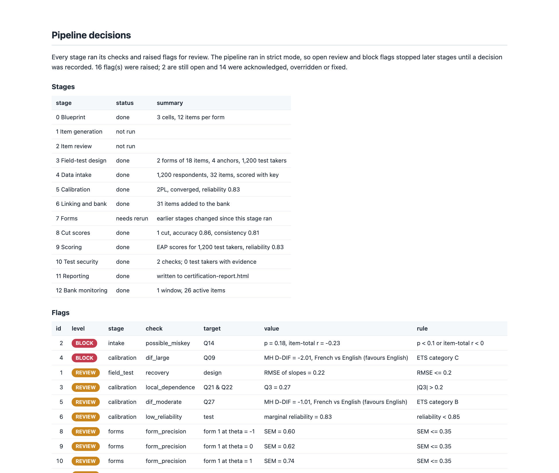
Figure 3: The pipeline decisions section of the technical report created by pipeline_report()

The pipeline also keeps the R code for every step in p$code. Here are the first few lines:

cat(head(p$code, 8), sep = "\n")

library(mirtverse)
p <- mv_pipeline(title = "Certification exam", strict = TRUE, verbose = FALSE)
p <- set_blueprint(p, cells = c(Ethics = 4, Practice = 5, Law = 3), construct = "Professional knowledge for certification", 
    use = "pass/fail certification", reliability = 0.85)
p <- design_field_test(p, n_forms = 2, n_per_form = 600, items = 32, reps = 2, seed = 1)
p <- acknowledge(p, check = "recovery", note = "Sample fixed by the testing window")
p <- add_responses(p, data = certexam, items = 3:34, key = certexam_key, group = "language", 
    id = "id")
p <- drop_items(p, items = "Q14", note = "Key confirmed wrong by the item writer")
p <- calibrate(p, model = "2PL")

This means that the entire pipeline, including every human decision and its reason, can be rerun from a single script.

Stage 12: Bank Monitoring

The work does not end when the scores are reported. After each administration, monitor_bank() records the administration in the bank under a window name and checks the bank’s history: items over-exposed in consecutive windows, content cells with too few active items, reliability falling from its first value, and items unused for a year.

p <- monitor_bank(p, window = "2026 spring", date = "2026-04-15",
                  content = content)
p$monitoring$cells

# A tibble: 3 × 3
  cell     active minimum
  <chr>     <int>   <dbl>
1 Ethics       10       8
2 Practice     11      10
3 Law          10       6

The minimum column comes from the blueprint: by default, the bank should hold at least twice as many active items in each cell as a single form needs. Now, suppose that even though we found no evidence of preknowledge, the testing board decides to retire the five items posted on the study forum as a precaution. retire_items() keeps the items in the bank with their history but stops using them for forms and linking.

p <- retire_items(p, c("Q01", "Q02", "Q03", "Q04", "Q05"),
                  note = "Posted on a study forum; retired as a precaution")
p <- monitor_bank(p, record = FALSE)
flags(p, stage = "monitoring") %>% select(check, target, value, advice)

# A tibble: 1 × 4
  check      target value                      
  <chr>      <chr>  <chr>                      
1 bank_depth Ethics 5 active item(s), minimum 8
  advice                                                              
  <chr>                                                               
1 Write and field-test new items for this cell before more items are …

All five retired items were Ethics items, so the Ethics cell now has only five active items, which is below the minimum of eight. The gate turns a human decision at one stage (retiring items) into a concrete task for another stage (writing new Ethics items). Retiring items also marks the forms as needing a rerun, which we will see in the next section.

Where Everything Stands

At any point, printing the pipeline shows each stage, its summary, and its open flags:

p

<mv_pipeline> Certification exam
strict: open review and block flags stop the next stage; rules: standards

[x] 0  Blueprint         3 cells, 12 items per form
[ ] 1  Item generation   not run
[ ] 2  Item review       not run
[x] 3  Field-test design 2 forms of 18 items, 4 anchors, 1,200 test takers
[x] 4  Data intake       1,200 respondents, 32 items, scored with key
[x] 5  Calibration       2PL, converged, reliability 0.83  | open: 1 info
[x] 6  Linking and bank  31 items added to the bank
[!] 7  Forms             earlier stages changed since this stage ran
[x] 8  Cut scores        1 cut, accuracy 0.86, consistency 0.81
[x] 9  Scoring           EAP scores for 1,200 test takers, reliability 0.83
[x] 10 Test security     2 checks; 0 test takers with evidence
[x] 11 Reporting         written to certification-report.html
[x] 12 Bank monitoring   1 window, 26 active items  | open: 1 review

Open flags: 1 review, 1 info. See flags(p). 14 decision(s) recorded.

Finally, let’s look at all the flags raised during the pipeline and how they were resolved. flags(p, status = "all") returns the open flags together with the ones that have already been decided.

stage_order <- c("field_test", "intake", "calibration", "forms",
                 "cuts", "scoring", "monitoring")

flags(p, status = "all") %>%
  mutate(stage = factor(stage, levels = stage_order),
         status = factor(status, levels = c("fixed", "overridden", "acknowledged", "open"))) %>%
  count(stage, status) %>%
  ggplot(aes(x = stage, y = n, fill = status)) +
  geom_col(width = 0.65) +
  scale_fill_manual(values = c(fixed = "#1baf7a", overridden = "#eb6834",
                               acknowledged = "#2a78d6", open = "grey70")) +
  labs(x = "Pipeline stage", y = "Number of flags", fill = NULL) +
  theme_blog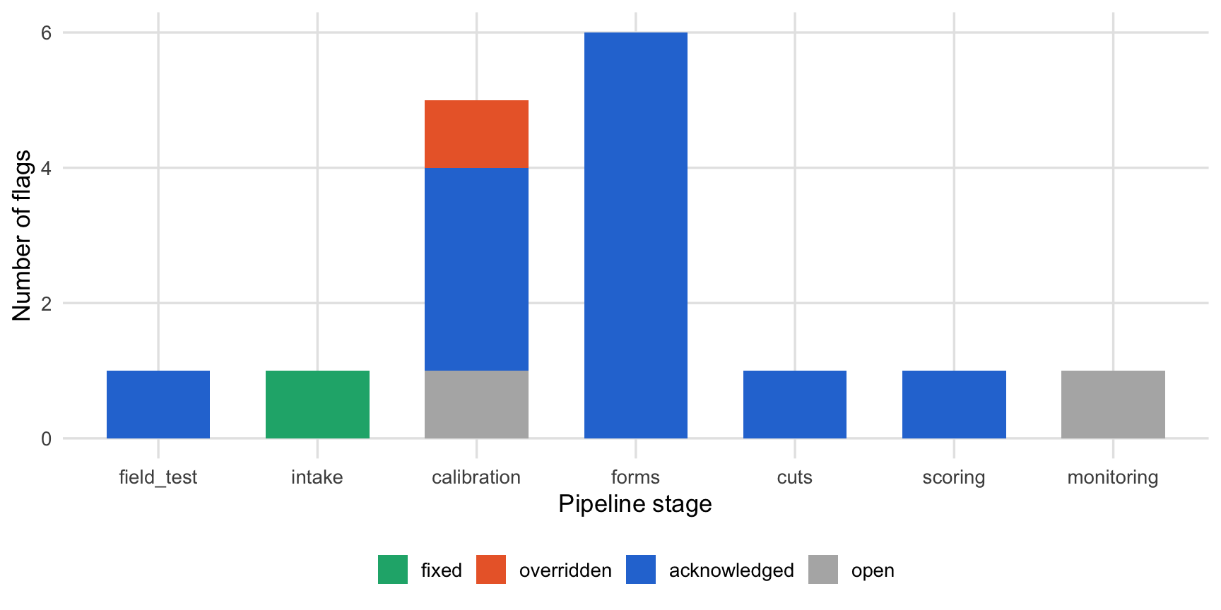

Figure 4: Flags raised by each stage and how they were resolved

In total, the gates raised 16 flags. One was fixed by removing an item, one block flag was overridden with a written reason, 12 were acknowledged with notes, and two are still open: the person misfit flag (for awareness only) and the shortage of Ethics items in the bank, which is the next task for the item writers. Every one of these decisions was made by a person, and every one of them is on record.

The Pipeline in the Workbench

Not everyone who makes these decisions writes R code. For this reason, the point-and-click workbench in mirtverse (launch_workbench()) has a Pipeline tab. It can run uploaded data through the intake and calibration gates or load a pipeline saved with saveRDS(). The tab shows the stage tracker and the flags, lets users select flags to acknowledge, override, or drop items, and then recalibrates the model. Like the rest of the workbench, it shows the R code for every step, so a content expert can record decisions in the app and a psychometrician can rerun the same pipeline from the code.

Concluding Remarks

In this post, I argued that test development needs assessment pipelines that automate routine psychometric checks but leave the decisions to people, and I introduced the assessment pipeline in mirtverse. Here are the main takeaways:

1. Every stage has a gate. The 13 stages of the pipeline, from the blueprint to bank monitoring, each end with checks that compare the results with explicit thresholds in mv_rules().
2. Flags are graded. Info, review, and block flags separate what is worth knowing from what needs attention and what makes later stages unsafe.
3. Humans make the decisions. acknowledge(), override(), and drop_items() record each decision and its reason next to the evidence. Language models can draft items or screen them for bias, but human reviewers decide.
4. Strict mode prevents silent failures. In high-stakes settings, the pipeline refuses to continue while serious flags are open, as we saw with the miskeyed item.
5. Everything is reproducible. The technical report lists every flag and decision, and p$code reruns the whole pipeline.

The assessment pipeline is the newest part of mirtverse, and this is its first phase. I plan to extend it in future versions, so I would very much like to hear from people who develop tests about which checks and stages matter most in their work. You can open an issue on GitHub or read the full article, An assessment pipeline from blueprint to bank monitoring, on the package website. Happy testing!