Okan Bulut: Introduction to Psychometric Network Analysis

Okan Bulut

Introduction

Psychometric Network Analysis (PNA), which is also referred to as “network psychometrics”, is an emerging field that combines concepts from psychometrics and network analysis to study the relationships among psychological variables. Generally, psychometrics involves the measurement of latent traits, while network analysis focuses on modeling and analyzing complex systems of interconnected elements. PNA aims to represent the relationships between psychological constructs, such as symptoms, traits, or behaviors, as a network of interconnected nodes. The figure below shows a network graph for the Big Five Personality Test:

Figure from [Epskamp (2017)](https://hdl.handle.net/11245.1/a76273c6-6abc-4cc7-a2e9-3b5f1ae3c29e)

Figure 1: Figure from Epskamp (2017)

Each node represents a specific personality trait, and the edges (connections) between nodes reflect the statistical relationships between those variables. The edges can be weighted to represent the strength (e.g., thicker edges represents stronger associations) and direction of the relationships between the corresponding traits (e.g., green lines for positive and red lines for negative associations).

In social sciences (especially in psychology and education), researchers often use “partial correlation” coefficients to understand the associations between the variables. A partial correlation is the association between two [quantitative] variables, after conditioning on all other variables in the dataset. Networks based on partial correlations are known as Gaussian Graphical Models (GGMs; Costantini et al. (2015)). A GGM can be mathematically expressed as follows:

\[Σ=Δ(I−Ω)^{−1}Δ,\] where \(Σ\) is the variance-covariance matrix of the observed variables, \(Δ\) is a diagonal matrix, \(Ω\) is a matrix containing weights linking observed variables, conditioned on all other variables, and \(I\) is the identity matrix.

To prevent over-interpretation in network structures, we want to limit the number of spurious connections (i.e., weak partial correlations due to sampling variation). It is possible to eliminate spurious connections using statistical regularization techniques, such as “least absolute shrinkage and selection operator” (LASSO; Tibshirani (1996)). LASSO (L1) regularization shrinks partial correlation coefficients when estimating a network model, which means that small coefficients are estimated to be exactly zero.

As an extension of LASSO, graphical LASSO, or shortly glasso (Friedman et al., 2007), involves a penalty parameter (\(\lambda\)) to remove weak associations within a network. The following figure demonstrates the impact of the penalty parameter.

Figure Adapted from [Epskamp and Fried (2017)](https://doi.org/10.1037/met0000167)

Figure 2: Figure Adapted from Epskamp and Fried (2017)

When estimating network models, glasso is typically combined with the extended Bayesian information criterion (EBIC; Chen & Chen (2008)) for tuning parameter selection, resulting in EBICglasso (Epskamp & Fried, 2018). If the dataset for PNA consists of continuous variables that are multivariate normally distributed, then we can estimate a GGM based on partial correlations with glasso or EBICglasso. GGM can also be used for ordinal data (e.g., Likert-scale data) wherein the network is based on the polychoric correlations instead of partial correlations.

In this blog post, I want to demonstrate how to perform PNA and visualize resulting network models (specifically, GGMs) using R 🕸 👩‍💻. I highly encourage readers to check out Network Psychometrics with R by Isvoranu et al. (2022) for a comprehensive discussion of network models and their estimation using R.

Let’s get started 💪.

Example

In our example, we will use a subset of the Synthetic Aperture Personality Assessment (SAPA)–a web based personality assessment project (https://www.sapa-project.org/). The purpose of SAPA is to find patterns among the vast number of ways that people differ from one another in terms of their thoughts, feelings, interests, abilities, desires, values, and preferences (Condon & Revelle, 2014; Revelle et al., 2010). The dataset consists of 16 SAPA items sampled from the full instrument (80 items). These items measure four subskills (i.e., verbal reasoning, letter series, matrix reasoning, and spatial rotations) as part of the general intelligence, also known as g factor. The “sapa_data.csv” dataset is a data frame with 1525 individuals who responded to 16 multiple-choice items in SAPA. The original dataset is included in the psych package (William Revelle, 2023). The dataset can be downloaded from here. Now, let’s import the data into R and then review its content.

# Read the data in R
sapa <- read.csv("sapa_data.csv", header = TRUE)

# Preview the data
head(data)

Next, we will check out the correlations among the SAPA items. Since the items are dichotomous (i.e., binary), we will compute the tetrachoric correlations and then visualize the matrix using a correlation matrix plot.

library("psych")
library("ggcorrplot")  

# Save the correlation matrix
cormat <- psych::tetrachoric(x = sapa)$rho

# Correlation matrix plot
ggcorrplot::ggcorrplot(corr = cormat, # correlation matrix
                       type = "lower", # print only the lower part of the correlation matrix
                       hc.order = TRUE, # hierarchical clustering
                       show.diag = TRUE, # show the diagonal values of 1
                       lab = TRUE, # add correlation values as labels
                       lab_size = 3) # Size of the labels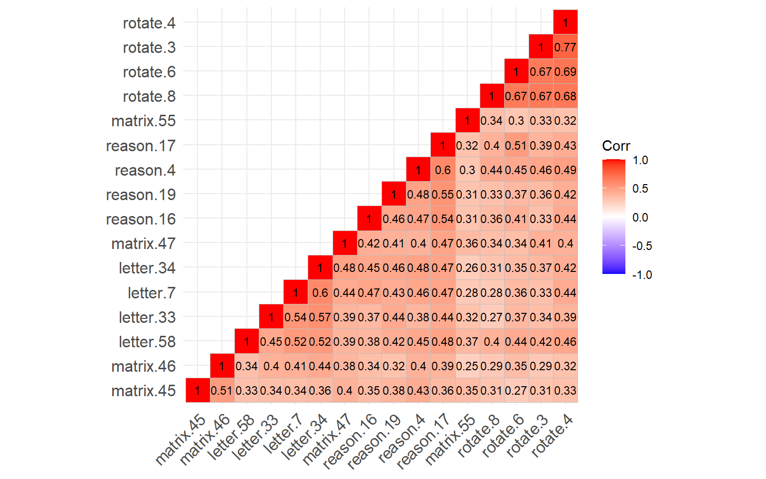

Figure 3: Correlation matrix plot of the SAPA items

The figure above shows that all of the SAPA items are positively correlated with each other. the items associated with the same construct (e.g., rotation) seem to have been clustered together (e.g., see the rotate.4, rotate.3, rotate.6, and rotate.8 as the top cluster). Now, we can go ahead and estimate a GGM based on this correlation matrix.

We will use the bootnet package (Epskamp, Borsboom, et al., 2018). This package has many methods to estimate GGMs. In our example, we will use “IsingFit” because the Ising model deal with binary data (see Epskamp, Maris, et al. (2018) and Marsman et al. (2018) for more details on the Ising network models). This model combines L1-regularized logistic regression with model selection based on EBIC.

library("bootnet")

network_sapa_1 <- bootnet::estimateNetwork(
  data = sapa, # dataset
  default = "IsingFit", # for estimating GGM with the Ising model and EBIC,
  verbose = FALSE # Ignore real-time updates on the estimation process
)

# View the estimated network
plot(network_sapa_1, layout = "spring")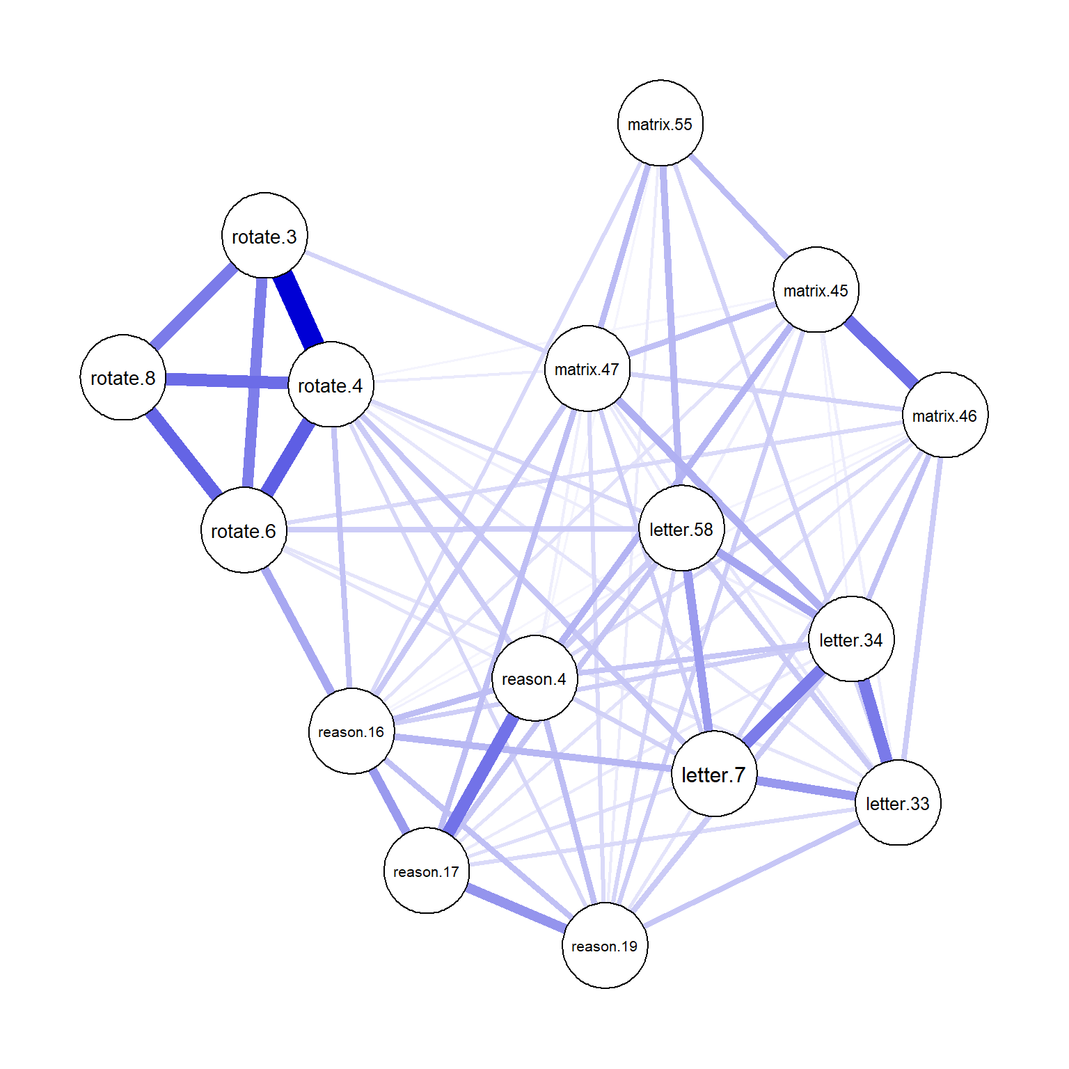

Figure 4: Network plot for the Ising model

From the network plot above, we can see that the items associated with the same construct often have stronger edges between the nodes (e.g., see the thick edges between the rotation items). These items also appear to be clustered closely within the network.

What if we compute the polychoric correlations for the SAPA items using corMethod = "cor_auto" and estimate a GGM with glasso and EBIC?

network_sapa_2 <- bootnet::estimateNetwork(
  data = sapa,
  corMethod = "cor_auto", # for polychoric correlations
  default = "EBICglasso", # for estimating GGM with glasso and EBIC
  verbose = FALSE
)

# View the estimated network
plot(network_sapa_2, layout = "spring")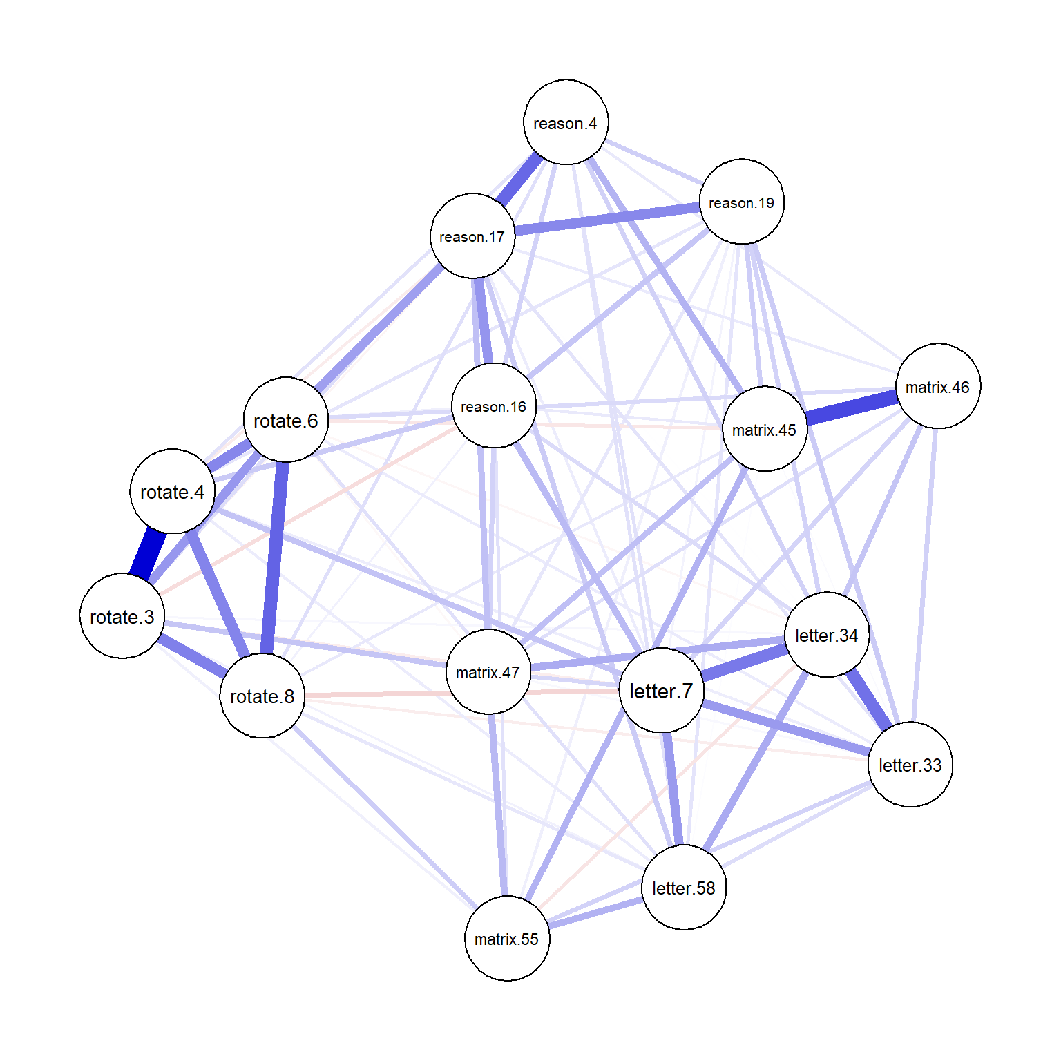

Figure 5: Network plot for the GGM

By default, the bootnet package uses tuning = 0.5 for the penalty parameter for EBICglasso. We can increase or decrease this parameter to adjust the penalty on the model (Note: tuning = 0 leads to model selection based on BIC instead of EBIC). In the following example, we will use tuning = 1 to apply a larger penalty parameter to the model.

network_sapa_3 <- bootnet::estimateNetwork(
  data = sapa,
  corMethod = "cor_auto", # for polychoric correlations
  default = "EBICglasso", # for estimating GGM with glasso and EBIC
  tuning = 1, 
  verbose = FALSE
)

# View the estimated network
plot(network_sapa_3, layout = "spring")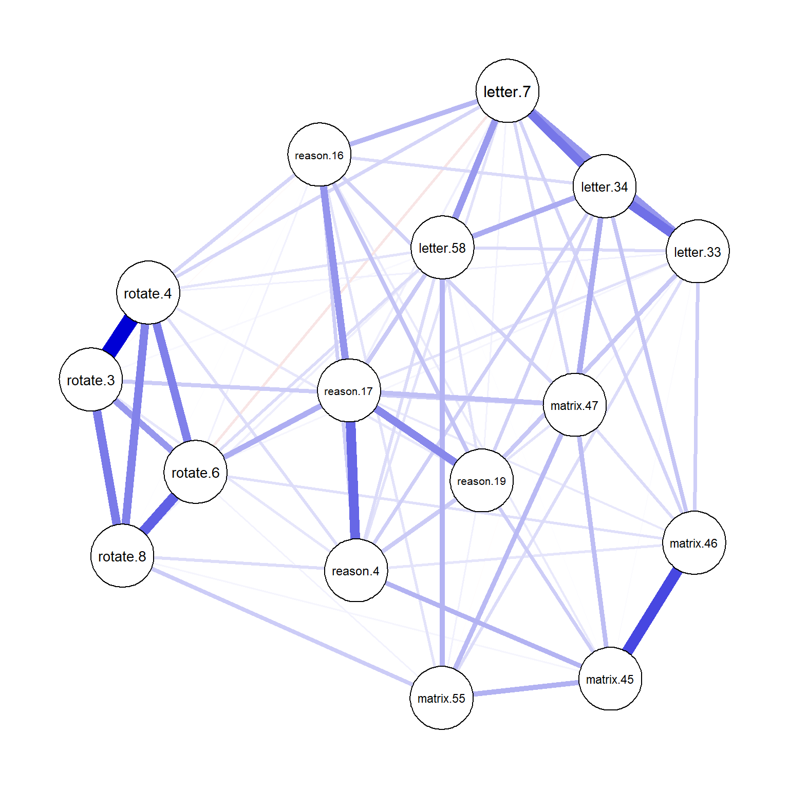

Figure 6: Network plot for the GGM after tuning

The final network plot includes fewer edges compared to the previous one with the default tuning parameter of 0.5. As the tuning parameter gets larger, more edges may be eliminated from the network, leading to a more compact and interpretable model.

I also want to demonstrate the same analysis using the psychonetrics package (Epskamp, 2023). This package is more versatile than bootnet as it is capable of estimating both network models and structural equation models.

library("psychonetrics")
library("dplyr")

network_sapa_4 <- psychonetrics::ggm(data = sapa,
                                     omega = "full", # or "empty" to set all elements to zero
                                     delta = "full", # or "empty" to set all elements to zero
                                     estimator = "FIML", # or "ML", "ULS", or "DWLS"
                                     verbose = FALSE) %>%
  psychonetrics::runmodel() # Run the model

# View the model parameters
network_sapa_4 %>% 
  psychonetrics::parameters()


 Parameters for group fullsample
    -  mu  
      var1 op var2  est     se        p row col par
  reason.4 ~1      0.64  0.012 < 0.0001   1   1   1
 reason.16 ~1      0.70  0.012 < 0.0001   2   1   2
 reason.17 ~1      0.70  0.012 < 0.0001   3   1   3
 reason.19 ~1      0.62  0.012 < 0.0001   4   1   4
  letter.7 ~1      0.60  0.013 < 0.0001   5   1   5
 letter.33 ~1      0.57  0.013 < 0.0001   6   1   6
 letter.34 ~1      0.61  0.012 < 0.0001   7   1   7
 letter.58 ~1      0.44  0.013 < 0.0001   8   1   8
 matrix.45 ~1      0.53  0.013 < 0.0001   9   1   9
 matrix.46 ~1      0.55  0.013 < 0.0001  10   1  10
 matrix.47 ~1      0.61  0.012 < 0.0001  11   1  11
 matrix.55 ~1      0.37  0.012 < 0.0001  12   1  12
  rotate.3 ~1      0.19  0.010 < 0.0001  13   1  13
  rotate.4 ~1      0.21  0.010 < 0.0001  14   1  14
  rotate.6 ~1      0.30  0.012 < 0.0001  15   1  15
  rotate.8 ~1      0.19 0.0099 < 0.0001  16   1  16

    -  omega (symmetric) 
      var1 op      var2     est    se        p row col par
 reason.16 --  reason.4   0.086 0.025  0.00072   2   1  17
 reason.17 --  reason.4    0.20 0.025 < 0.0001   3   1  18
 reason.19 --  reason.4   0.091 0.025  0.00034   4   1  19
  letter.7 --  reason.4   0.064 0.026    0.012   5   1  20
 letter.33 --  reason.4  0.0015 0.026     0.95   6   1  21
 letter.34 --  reason.4   0.077 0.025   0.0024   7   1  22
 letter.58 --  reason.4   0.060 0.026    0.018   8   1  23
 matrix.45 --  reason.4    0.10 0.025 < 0.0001   9   1  24
 matrix.46 --  reason.4   0.054 0.026    0.033  10   1  25
 matrix.47 --  reason.4   0.025 0.026     0.33  11   1  26
 matrix.55 --  reason.4   0.013 0.026     0.61  12   1  27
  rotate.3 --  reason.4   0.037 0.026     0.14  13   1  28
  rotate.4 --  reason.4   0.034 0.026     0.18  14   1  29
  rotate.6 --  reason.4   0.035 0.026     0.17  15   1  30
  rotate.8 --  reason.4   0.034 0.026     0.19  16   1  31
 reason.17 -- reason.16    0.15 0.025 < 0.0001   3   2  32
 reason.19 -- reason.16   0.090 0.025  0.00041   4   2  33
  letter.7 -- reason.16   0.097 0.025  0.00014   5   2  34
 letter.33 -- reason.16   0.018 0.026     0.48   6   2  35
 letter.34 -- reason.16   0.066 0.026    0.010   7   2  36
 letter.58 -- reason.16  0.0081 0.026     0.75   8   2  37
 matrix.45 -- reason.16   0.042 0.026    0.098   9   2  38
 matrix.46 -- reason.16   0.021 0.026     0.41  10   2  39
 matrix.47 -- reason.16   0.073 0.025   0.0039  11   2  40
 matrix.55 -- reason.16   0.046 0.026    0.074  12   2  41
  rotate.3 -- reason.16  -0.027 0.026     0.30  13   2  42
  rotate.4 -- reason.16   0.040 0.026     0.12  14   2  43
  rotate.6 -- reason.16   0.043 0.026    0.094  15   2  44
  rotate.8 -- reason.16   0.020 0.026     0.43  16   2  45
 reason.19 -- reason.17    0.15 0.025 < 0.0001   4   3  46
  letter.7 -- reason.17   0.049 0.026    0.055   5   3  47
 letter.33 -- reason.17   0.055 0.026    0.031   6   3  48
 letter.34 -- reason.17   0.037 0.026     0.14   7   3  49
 letter.58 -- reason.17   0.068 0.026   0.0079   8   3  50
 matrix.45 -- reason.17  0.0052 0.026     0.84   9   3  51
 matrix.46 -- reason.17   0.046 0.026    0.075  10   3  52
 matrix.47 -- reason.17   0.092 0.025  0.00030  11   3  53
 matrix.55 -- reason.17   0.017 0.026     0.50  12   3  54
  rotate.3 -- reason.17  -0.011 0.026     0.66  13   3  55
  rotate.4 -- reason.17  -0.021 0.026     0.40  14   3  56
  rotate.6 -- reason.17   0.092 0.025  0.00030  15   3  57
  rotate.8 -- reason.17   0.012 0.026     0.64  16   3  58
  letter.7 -- reason.19   0.045 0.026    0.078   5   4  59
 letter.33 -- reason.19   0.081 0.025   0.0015   6   4  60
 letter.34 -- reason.19   0.074 0.025   0.0039   7   4  61
 letter.58 -- reason.19   0.054 0.026    0.035   8   4  62
 matrix.45 -- reason.19   0.076 0.025   0.0030   9   4  63
 matrix.46 -- reason.19 0.00040 0.026     0.99  10   4  64
 matrix.47 -- reason.19   0.055 0.026    0.031  11   4  65
 matrix.55 -- reason.19   0.036 0.026     0.16  12   4  66
  rotate.3 -- reason.19   0.013 0.026     0.60  13   4  67
  rotate.4 -- reason.19   0.034 0.026     0.19  14   4  68
  rotate.6 -- reason.19   0.014 0.026     0.57  15   4  69
  rotate.8 -- reason.19  0.0054 0.026     0.83  16   4  70
 letter.33 --  letter.7    0.14 0.025 < 0.0001   6   5  71
 letter.34 --  letter.7    0.18 0.025 < 0.0001   7   5  72
 letter.58 --  letter.7    0.13 0.025 < 0.0001   8   5  73
 matrix.45 --  letter.7   0.013 0.026     0.60   9   5  74
 matrix.46 --  letter.7   0.070 0.025   0.0063  10   5  75
 matrix.47 --  letter.7   0.072 0.025   0.0049  11   5  76
 matrix.55 --  letter.7  0.0072 0.026     0.78  12   5  77
  rotate.3 --  letter.7  -0.018 0.026     0.48  13   5  78
  rotate.4 --  letter.7   0.060 0.026    0.019  14   5  79
  rotate.6 --  letter.7   0.013 0.026     0.63  15   5  80
  rotate.8 --  letter.7  -0.031 0.026     0.23  16   5  81
 letter.34 -- letter.33    0.18 0.025 < 0.0001   7   6  82
 letter.58 -- letter.33   0.070 0.025   0.0059   8   6  83
 matrix.45 -- letter.33   0.030 0.026     0.25   9   6  84
 matrix.46 -- letter.33   0.075 0.025   0.0034  10   6  85
 matrix.47 -- letter.33   0.038 0.026     0.14  11   6  86
 matrix.55 -- letter.33   0.063 0.026    0.013  12   6  87
  rotate.3 -- letter.33   0.013 0.026     0.61  13   6  88
  rotate.4 -- letter.33   0.029 0.026     0.26  14   6  89
  rotate.6 -- letter.33   0.044 0.026    0.087  15   6  90
  rotate.8 -- letter.33  -0.025 0.026     0.32  16   6  91
 letter.58 -- letter.34    0.11 0.025 < 0.0001   8   7  92
 matrix.45 -- letter.34   0.023 0.026     0.37   9   7  93
 matrix.46 -- letter.34   0.084 0.025  0.00092  10   7  94
 matrix.47 -- letter.34    0.11 0.025 < 0.0001  11   7  95
 matrix.55 -- letter.34  -0.027 0.026     0.30  12   7  96
  rotate.3 -- letter.34   0.024 0.026     0.35  13   7  97
  rotate.4 -- letter.34   0.014 0.026     0.59  14   7  98
  rotate.6 -- letter.34  -0.014 0.026     0.58  15   7  99
  rotate.8 -- letter.34 -0.0020 0.026     0.94  16   7 100
 matrix.45 -- letter.58   0.026 0.026     0.32   9   8 101
 matrix.46 -- letter.58   0.021 0.026     0.42  10   8 102
 matrix.47 -- letter.58   0.026 0.026     0.31  11   8 103
 matrix.55 -- letter.58    0.10 0.025 < 0.0001  12   8 104
  rotate.3 -- letter.58   0.032 0.026     0.21  13   8 105
  rotate.4 -- letter.58   0.046 0.026    0.073  14   8 106
  rotate.6 -- letter.58   0.069 0.026   0.0065  15   8 107
  rotate.8 -- letter.58   0.039 0.026     0.12  16   8 108
 matrix.46 -- matrix.45    0.22 0.024 < 0.0001  10   9 109
 matrix.47 -- matrix.45   0.089 0.025  0.00049  11   9 110
 matrix.55 -- matrix.45    0.10 0.025 < 0.0001  12   9 111
  rotate.3 -- matrix.45   0.018 0.026     0.49  13   9 112
  rotate.4 -- matrix.45   0.017 0.026     0.51  14   9 113
  rotate.6 -- matrix.45  -0.027 0.026     0.29  15   9 114
  rotate.8 -- matrix.45   0.032 0.026     0.21  16   9 115
 matrix.47 -- matrix.46   0.063 0.026    0.013  11  10 116
 matrix.55 -- matrix.46   0.011 0.026     0.68  12  10 117
  rotate.3 -- matrix.46 -0.0057 0.026     0.82  13  10 118
  rotate.4 -- matrix.46  0.0016 0.026     0.95  14  10 119
  rotate.6 -- matrix.46   0.062 0.026    0.015  15  10 120
  rotate.8 -- matrix.46   0.013 0.026     0.61  16  10 121
 matrix.55 -- matrix.47   0.089 0.025  0.00045  12  11 122
  rotate.3 -- matrix.47   0.054 0.026    0.036  13  11 123
  rotate.4 -- matrix.47   0.017 0.026     0.50  14  11 124
  rotate.6 -- matrix.47     ~ 0 0.026      1.0  15  11 125
  rotate.8 -- matrix.47   0.014 0.026     0.58  16  11 126
  rotate.3 -- matrix.55   0.038 0.026     0.14  13  12 127
  rotate.4 -- matrix.55   0.014 0.026     0.59  14  12 128
  rotate.6 -- matrix.55   0.019 0.026     0.45  15  12 129
  rotate.8 -- matrix.55   0.063 0.026    0.013  16  12 130
  rotate.4 --  rotate.3    0.33 0.023 < 0.0001  14  13 131
  rotate.6 --  rotate.3    0.16 0.025 < 0.0001  15  13 132
  rotate.8 --  rotate.3    0.19 0.025 < 0.0001  16  13 133
  rotate.6 --  rotate.4    0.19 0.025 < 0.0001  15  14 134
  rotate.8 --  rotate.4    0.19 0.025 < 0.0001  16  14 135
  rotate.8 --  rotate.6    0.20 0.025 < 0.0001  16  15 136

    -  delta (diagonal) 
      var1  op      var2  est     se        p row col par
  reason.4 ~/~  reason.4 0.41 0.0074 < 0.0001   1   1 137
 reason.16 ~/~ reason.16 0.40 0.0073 < 0.0001   2   2 138
 reason.17 ~/~ reason.17 0.38 0.0070 < 0.0001   3   3 139
 reason.19 ~/~ reason.19 0.42 0.0077 < 0.0001   4   4 140
  letter.7 ~/~  letter.7 0.41 0.0075 < 0.0001   5   5 141
 letter.33 ~/~ letter.33 0.43 0.0078 < 0.0001   6   6 142
 letter.34 ~/~ letter.34 0.40 0.0073 < 0.0001   7   7 143
 letter.58 ~/~ letter.58 0.43 0.0078 < 0.0001   8   8 144
 matrix.45 ~/~ matrix.45 0.44 0.0081 < 0.0001   9   9 145
 matrix.46 ~/~ matrix.46 0.44 0.0080 < 0.0001  10  10 146
 matrix.47 ~/~ matrix.47 0.43 0.0078 < 0.0001  11  11 147
 matrix.55 ~/~ matrix.55 0.45 0.0082 < 0.0001  12  12 148
  rotate.3 ~/~  rotate.3 0.32 0.0057 < 0.0001  13  13 149
  rotate.4 ~/~  rotate.4 0.32 0.0058 < 0.0001  14  14 150
  rotate.6 ~/~  rotate.6 0.38 0.0068 < 0.0001  15  15 151
  rotate.8 ~/~  rotate.8 0.33 0.0059 < 0.0001  16  16 152

We can also see some information on the model fit, which can be used for making comparisons if we make any changes to the model (e.g., pruning).

# Look at the model fit
network_sapa_4 %>% 
  psychonetrics::fit()

           Measure     Value
              logl -13298.10
 unrestricted.logl -13298.10
     baseline.logl -15949.45
              nvar        16
              nobs       152
              npar       152
                df       ~ 0
         objective    -11.94
             chisq       ~ 0
            pvalue         1
    baseline.chisq   5302.71
       baseline.df       120
   baseline.pvalue       ~ 0
               nfi         1
              pnfi       ~ 0
               tli          
              nnfi         1
               rfi          
               ifi         1
               rni         1
               cfi         1
             rmsea          
    rmsea.ci.lower       ~ 0
    rmsea.ci.upper       ~ 0
      rmsea.pvalue       ~ 0
            aic.ll  26900.19
           aic.ll2  26934.10
             aic.x       ~ 0
            aic.x2       304
               bic  27710.32
              bic2  27227.45
           ebic.25  28131.75
            ebic.5  28553.18
           ebic.75  28890.33
             ebic1  29396.05

Another important feature of the ggm() function is that statistically insignificant edges can be removed to have a more compact model. In the following codes, we will eliminate edges that are not statistically significant at the alpha level of \(\alpha = .05\), after performing a Benjamini and Hochberg (known as “BH” or “fdr”) correction (Benjamini & Hochberg, 1995). We will then compare this model with the previous model.

# We can prune this model to remove insignificant edges
network_sapa_5 <- psychonetrics::ggm(data = sapa,
                                     omega = "full", # or "empty" to set all elements to zero
                                     delta = "full", # or "empty" to set all elements to zero
                                     estimator = "FIML", # or "ML", "ULS", or "DWLS"
                                     verbose = FALSE) %>%
  psychonetrics::runmodel() %>%
  psychonetrics::prune(adjust = "fdr", alpha = 0.05)

# Compare the models
comparison <- psychonetrics::compare(
  `1. Original model`  = network_sapa_4,
  `2. Compact model after pruning` = network_sapa_5)

print(comparison)

                          model DF      AIC      BIC RMSEA  Chisq
              1. Original model  0 26900.19 27710.32          ~ 0
 2. Compact model after pruning 73 26985.28 27406.33 0.038 231.09
 Chisq_diff DF_diff  p_value
                            
     231.09      73 < 0.0001

Note: Chi-square difference test assumes models are nested.

The results show that the compact model with pruning fits the data better based on BIC although AIC shows the opposite result. In the final step, we will visualize the last network model resulting from ggm() using the famous qgraph package (Epskamp et al., 2012):

library("qgraph")

# Obtain the network plot
net5 <- getmatrix(network_sapa_5, "omega")

qgraph::qgraph(net5, 
               layout = "spring", 
               theme = "colorblind",
               labels = colnames(sapa))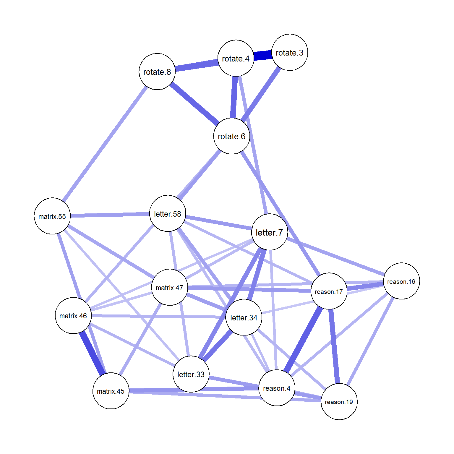

Figure 7: Network plot using qgraph

Conclusion

This was a very brief introduction to PNA using R. There are still many things to discuss in PNA. Thus, I plan to write several blog posts on PNA over the next few months. For example, I want to discuss centrality indices and demonstrate how to generate centrality indices for network models using R. I will also write a post on the Ising model for binary data to demonstrate the similarities and differences between an Ising network model and an item response theory (IRT) model.

Benjamini, Y., & Hochberg, Y. (1995). Controlling the false discovery rate: A practical and powerful approach to multiple testing. Journal of the Royal Statistical Society: Series B (Methodological), 57(1), 289–300. https://doi.org/https://doi.org/10.1111/j.2517-6161.1995.tb02031.x

Chen, J., & Chen, Z. (2008). Extended bayesian information criteria for model selection with large model spaces. Biometrika, 95(3), 759–771.

Condon, D. M., & Revelle, W. (2014). The international cognitive ability resource: Development and initial validation of a public-domain measure. Intelligence, 43, 52–64.

Costantini, G., Epskamp, S., Borsboom, D., Perugini, M., Mõttus, R., Waldorp, L. J., & Cramer, A. O. J. (2015). State of the aRt personality research: A tutorial on network analysis of personality data in r. Journal of Research in Personality, 54, 13–29. https://doi.org/https://doi.org/10.1016/j.jrp.2014.07.003

Epskamp, S. (2023). Psychonetrics: Structural equation modeling and confirmatory network analysis. https://CRAN.R-project.org/package=psychonetrics

Epskamp, S., Borsboom, D., & Fried, E. I. (2018). Estimating psychological networks and their accuracy: A tutorial paper. Behavior Research Methods, 50, 195–212.

Epskamp, S., Cramer, A. O. J., Waldorp, L. J., Schmittmann, V. D., & Borsboom, D. (2012). qgraph: Network visualizations of relationships in psychometric data. Journal of Statistical Software, 48(4), 1–18.

Epskamp, S., & Fried, E. I. (2018). A tutorial on regularized partial correlation networks. Psychological Methods, 23(4), 617.

Epskamp, S., Maris, G., Waldorp, L. J., & Borsboom, D. (2018). Network psychometrics. In The wiley handbook of psychometric testing (pp. 953–986). John Wiley & Sons, Ltd. https://doi.org/https://doi.org/10.1002/9781118489772.ch30

Friedman, J., Hastie, T., & Tibshirani, R. (2007). Sparse inverse covariance estimation with the graphical lasso. Biostatistics, 9(3), 432–441. https://doi.org/10.1093/biostatistics/kxm045

Isvoranu, A.-M., Epskamp, S., Waldorp, L., & Borsboom, D. (2022). Network psychometrics with r: A guide for behavioral and social scientists. Routledge.

Marsman, M., Borsboom, D., Kruis, J., Epskamp, S., Bork, R. van van, Waldorp, L., Maas, H. van der, & Maris, G. (2018). An introduction to network psychometrics: Relating ising network models to item response theory models. Multivariate Behavioral Research, 53(1), 15–35.

Revelle, W., Wilt, J., & Rosenthal, A. (2010). Individual differences in cognition: New methods for examining the personality-cognition link. In Handbook of individual differences in cognition (pp. 27–49). Springer.

Tibshirani, R. (1996). Regression shrinkage and selection via the lasso. Journal of the Royal Statistical Society. Series B (Methodological), 58(1), 267–288. http://www.jstor.org/stable/2346178

William Revelle. (2023). Psych: Procedures for psychological, psychometric, and personality research. Northwestern University. https://CRAN.R-project.org/package=psych

Comment on this article Share:

Introduction to Psychometric Network Analysis

Introduction

Example

Conclusion

References

Reuse

Citation