Introduction
Natural language processing (NLP) is a subfield of artificial intelligence that focuses on the linguistic interaction between humans and computers. Over the last two decades, NLP has been a rapidly growing field of research across many disciplines, yielding some advanced applications (e.g., automatic speech recognition, automatic translation of text, and chatbots). With the help of evolving machine learning and deep learning algorithms, NLP can help us systematically analyze large volumes of text data. The fundamental idea of NLP in various tasks stems from converting the natural language into a numerical format that computers can understand and process. This process is known as text vectorization. Effective and efficient vectorization of human language and text lays an important foundation to conduct advanced NLP tasks.
In this three-part series, we will explain text vectorization and demonstrate different methods for vectorizing textual data. First, we will begin with a basic vectorization approach that is widely used in text mining and NLP applications. More specifically, we will focus on how term-document matrices are constructed. In the following example, we will have a brief demonstration of this technique using Python 🐍 (instead of R)1.
Example
In this example, we will use a data set from one of the popular automated essay scoring competitions funded by the Hewlett Foundation: Short Answer Scoring. The data set includes students’ responses to a set of short-answer items and scores assigned by human raters. On average, each answer is approximately 50 words in length. The data set (train_rel_2.tsv) is available here as a tab-separated value (TSV) file. The data set consists of the following variables:
- Id: A unique identifier for each individual student essay.
- EssaySet: 1-10, an id for each set of essays.
- Score1: The human rater’s score for the answer. This is the final score for the answer and the score that you are trying to predict.
- Score2: A second human rater’s score for the answer. This is provided as a measure of reliability, but had no bearing on the score the essay received.
- EssayText: The ASCII text of a student’s response.
In this example, we will take a look at “Essay Set 1”, in which students were provided with a prompt describing a science experiment. The students were required to identify the missing information that is important to increase the replicability of the experiment procedures described in the prompt.
We will begin our analysis by importing the data set into Python.
# Import pandas for dataframe
# Import pprint for printing the outcomes
import pandas as pd
from pprint import pprint

# Import train_rel_2.tsv into Python
with open('train_rel_2.tsv', 'r') as f:
    lines = f.readlines()
    columns = lines[0].split('\t')
    data = []
    response_id= []
    score = []
    for line in lines[1:]:
        temp = line.split('\t')
        if temp[1] == '1':
            data.append(temp[-1])
            response_id.append(int(temp[0]))
            score.append(int(temp[2]))
        else:
            None

# Construct a dataframe ("doc") which includes the response_id, responses, and the score
doc = pd.DataFrame(list(zip(response_id, data, score)))
doc.columns = ['id', 'response', 'score']
Now, we can take a look at some of the student-written responses in the data set.
# Preview the first response in the data set
print('Sample response 1:')
pprint(doc.response.values[0])

# Preview the first 5 lines in the data set
doc.head(5)
Sample response 1:('Some additional information that we would need to replicate the experiment '
'is how much vinegar should be placed in each identical container, how or '
'what tool to use to measure the mass of the four different samples and how '
'much distilled water to use to rinse the four samples after taking them out '
'of the vinegar.\n') id response score
0 1 Some additional information that we would need... 1
1 2 After reading the expirement, I realized that ... 1
2 3 What you need is more trials, a control set up... 1
3 4 The student should list what rock is better an... 0
4 5 For the students to be able to make a replicat... 2Each student response is associated with a score ranging from 0 to 3, which indicates the overall quality of the response. For example, the first item in the data set focuses on science for Grade 10 students. The item requires students to identify the missing information that would allow replicating the experiment.
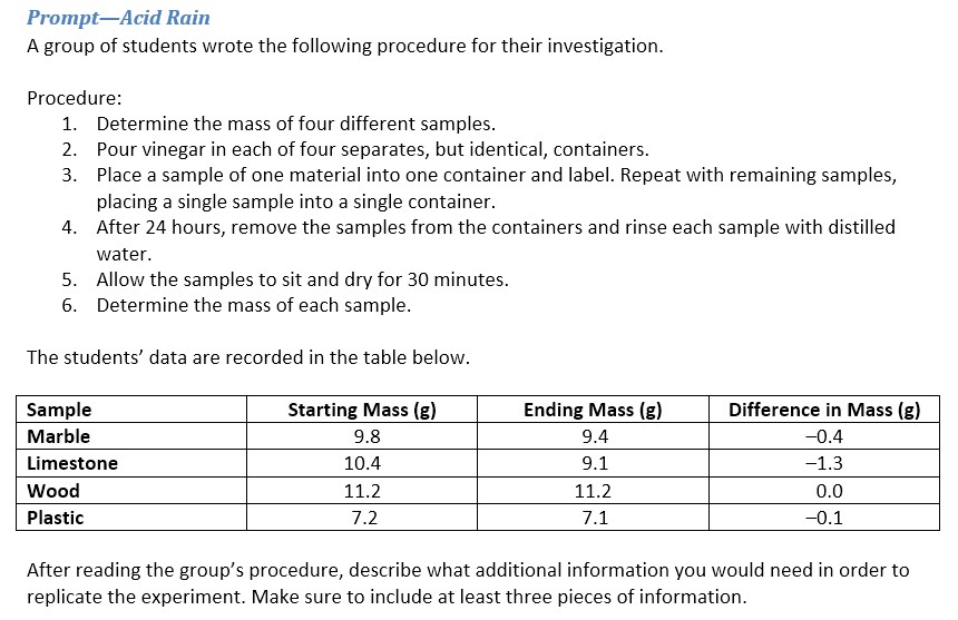
Figure 1: A preview of Essay Set 1 in the data set.
Each score (0, 1, 2, or 3 points) category contains a range of student responses which reflect the descriptions given below:
Score 3: The response is an excellent answer to the question. It is correct, complete, and appropriate and contains elaboration, extension, and evidence of higher-order thinking and relevant prior knowledge
Score 2: The response is a proficient answer to the question. It is generally correct, complete, and appropriate, although minor inaccuracies may appear. There may be limited evidence of elaboration, extension, higher-order thinking, and relevant prior knowledge.
Score 1: The response is a marginal answer to the question. While it may contain some elements of a proficient response, it is inaccurate, incomplete, or inappropriate.
Score 0: The response, though possibly on topic, is an unsatisfactory answer to the question. It may fail to address the question, or it may address the question in a very limited way.
By analyzing students’ responses to this item, we can find important hints from the vocabulary and word choices to better understand the overall quality of their responses. For example, score 3 indicates that the response is correct, complete, and appropriate and contains elaboration. To find out what an elaborate and complete response looks like, we will focus on the semantic structure of the responses.
Term-Document Matrix
Term-document matrix represents texts using the frequency of terms or words that appear in a set of documents. While the term-document matrix reveals information regarding most or least common words across multiple texts, little to no information is preserved regarding the order of how the words appear originally in the document (bag-of-words). Still, the term-document matrix provides important insights about the documents (also, it is very easy to construct and understand!)
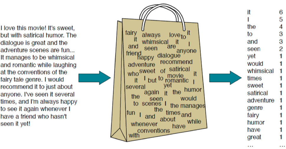
Figure 2: The illustration of the bag-of-words approach. (Source: http://people.cs.georgetown.edu/nschneid/cosc572/f16/05_classification-NB_slides.pdf).
We will use CountVectorizer to count how many times each unique word appears in the responses. For analytic simplicity, we will focus on the first five student responses and the top 25 words in this demonstration.
# Activate CountVectorizer
from sklearn.feature_extraction.text import CountVectorizer

# Count Vectorizer
vect = CountVectorizer()
vects = vect.fit_transform(doc.response)

# Select the first five rows from the data set
td = pd.DataFrame(vects.todense()).iloc[:5]
td.columns = vect.get_feature_names()
term_document_matrix = td.T
term_document_matrix.columns = ['Doc '+str(i) for i in range(1, 6)]
term_document_matrix['total_count'] = term_document_matrix.sum(axis=1)

# Top 25 words
term_document_matrix = term_document_matrix.sort_values(by ='total_count',ascending=False)[:25]

# Print the first 10 rows
print(term_document_matrix.drop(columns=['total_count']).head(10))
Doc 1 Doc 2 Doc 3 Doc 4 Doc 5
the 5 5 1 3 2
to 5 2 1 0 3
is 1 1 1 2 2
and 1 1 2 1 1
vinegar 2 1 1 0 1
what 1 0 1 2 1
you 0 3 2 0 0
of 2 1 1 0 1
how 3 0 0 0 1
in 1 1 1 1 0As the name suggests, each row in the term-document matrix indicates a unique word that appeared across the responses, while the columns represent a unique document (e.g., “Doc 1”, “Doc 2”, …) that are the responses for each student. Now let’s take a look at which words were most frequently used across the responses.
term_document_matrix['total_count'].plot.bar()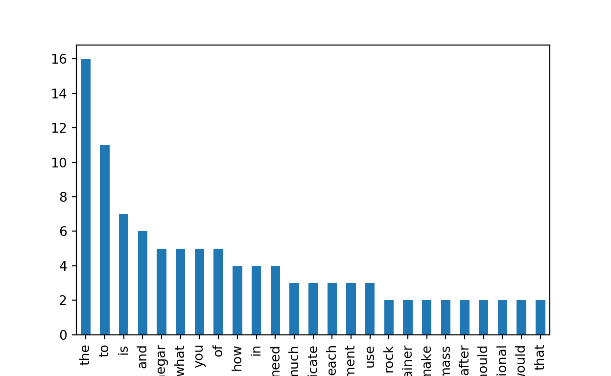
Figure 3: A bar plot of most frequent words in the responses.
Not surprisingly, the function words (e.g., “the”, “to”, “is”) appeared more frequently than other words with more contextual information, such as the words “rock”, “use”, and “mass”. Also, this unique distribution should remind us of a very famous distribution in linguistics: Unzipping Zipf’s Law.
Document-Term Vector Visualization
Now that we represented each document as a unique vector that indicates information regarding word occurrence, we can visualize the relationship between the documents. This can be easily achieved by simply getting a transpose of the term-document matrix (i.e., document-term matrix). Let’s use the two most frequent words “the” and “to” to plot the documents.
# Locate the and to in the documents
term_document_matrix.loc[['the', 'to']].T

# Create a scatterplot of the frequencies
the to
Doc 1 5 5
Doc 2 5 2
Doc 3 1 1
Doc 4 3 0
Doc 5 2 3
total_count 16 11term_document_matrix.drop(columns=['total_count']).T.plot.scatter(x='the', y='to')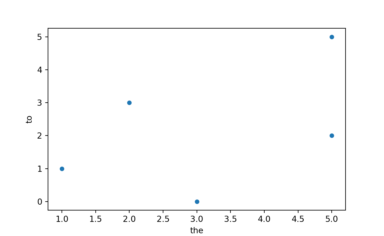
Figure 4: A scatterplot of frequencies for the and to across the first five documents.
It is quite difficult to understand which of the documents are highly related to each other just by looking at the relationships using two words. Now, we can plot the documents using the term vector to better understand the similarities (or differences) between their word distributions of the top 25 vocabularies that we selected above.
Cosine Similarity between Documents
We will use cosine similarity that evaluates the similarity between the two vectors by measuring the cosine angle between them. If the two vectors are in the same direction, hence similar, the similarity index yields a value close to 1. The cosine similarity index can be computed using the following formula:
\[ similarity = cos(\theta)=\frac{\mathbf{A}.\mathbf{B}}{\|\mathbf{A}\|\|\mathbf{B}\|}=\frac{\Sigma_{i=1}^nA_iB_i}{\sqrt{\Sigma_{i=1}^nA_i^2}\sqrt{\Sigma_{i=1}^nB_i^2}} \]
Now, let’s define a function to calculate cosine similarity between two vectors2:
# Activate math
import math

# Define a cosine similarity function
def cosine_similarity(a,b):
    "compute cosine similarity of v1 to v2: (a dot b)/{||a||*||b||)"
    sumxx, sumxy, sumyy = 0, 0, 0
    for i in range(len(a)):
        x = a[i]; y = b[i]
        sumxx += x*x
        sumyy += y*y
        sumxy += x*y
    return sumxy/math.sqrt(sumxx*sumyy)
Recall that each student response is associated with a score that represents the overall quality (or accuracy) of the response. We could hypothesize that for students who used similar words in their responses, the scores would be similar.
# Activate numpy
import numpy as np

# Save the similarity index between the documents
def pair(s):
    for i, v1 in enumerate(s):
        for j in range(i+1, len(s)):
            yield [v1, s[j]]

dic={}
for (a,b) in list(pair(['Doc 1', 'Doc 2', 'Doc 3', 'Doc 4', 'Doc 5'])):
  dic[(a,b)] = cosine_similarity(term_document_matrix[a].tolist(), term_document_matrix[b].tolist())

# Print the cosine similarity index
pprint(dic)
{('Doc 1', 'Doc 2'): 0.7003574164133837,
('Doc 1', 'Doc 3'): 0.5496565719302984,
('Doc 1', 'Doc 4'): 0.47601655464870696,
('Doc 1', 'Doc 5'): 0.8463976586173779,
('Doc 2', 'Doc 3'): 0.6674238124719146,
('Doc 2', 'Doc 4'): 0.5229577884350213,
('Doc 2', 'Doc 5'): 0.6510180115869747,
('Doc 3', 'Doc 4'): 0.4811252243246881,
('Doc 3', 'Doc 5'): 0.5689945423921311,
('Doc 4', 'Doc 5'): 0.4927637283262872}The values shown above indicate the similarity index for each document pair (i.e., student pairs). For example, the first row shows that the first document (i.e., student 1’s response) and the second document (i.e., student 2’s response) had a similarity index of 0.70. To see all the similarity indices together, we can create a heatmap that shows the cosine similarity index for each pair of documents.
documents= ['Doc 1', 'Doc 2', 'Doc 3', 'Doc 4', 'Doc 5']
final_df = pd.DataFrame(np.asarray([[(dic[(x,y)] if (x,y) in dic else 0) for y in documents] for x in documents]))
final_df.columns =  documents
final_df.index = documents

import matplotlib.pyplot as plt
fig, ax = plt.subplots()
ax.set_xticks(np.arange(len(documents)))
ax.set_yticks(np.arange(len(documents)))
ax.set_xticklabels(documents)
ax.set_yticklabels(documents)
ax.matshow(final_df, cmap='seismic')
for (i, j), z in np.ndenumerate(final_df):
  if z != 0 :
    ax.text(j, i, '{:0.2f}'.format(z), ha='center', va='center',
            bbox=dict(boxstyle='round', facecolor='white', edgecolor='0.3'))
  else:
    None
fig.suptitle('Cosine Similarity Index between the Documents')
plt.show()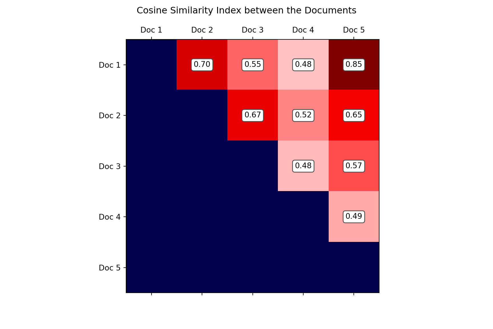
Figure 5: A heatmap of the cosine similarity indices across the five documents.
In our example, documents 1, 2, and 3 were scored as 1 point, document 4 was scored as 0 point, and document 5 was scored as 2 points. As shown in Figure 5, the highest similarity (0.85) occurs between Documents 1 and 5. This might be a surprising finding because these two documents were given different scores (1 and 2 points, respectively). In terms of the lowest similarity, we can see that document 4 is quite different from the rest of the documents with a relatively lower cosine similarity index (0.48, 0.52, and 0.48). This finding is not necessarily surprising because document 4 represents the only response scored as 0 points.
Conclusion
In this post, we demonstrated how we could convert text documents (e.g., a student’s written responses to an item) into a term-document matrix. Term-document vectorization is often called the “bag-of-words” representation (or shortly, BoW) as it focuses on considering the frequency of words in the document to understand and preserve its semantic representations. We also attempted to understand how we could use this vectorization approach to measure the similarities between the documents. In the next post, we will review how we can suppress the weights of “too frequently” occurring words, such as function words (e.g., “the”, “to”, “is”), using different vectorization approaches.
I plan to make a post showing the same analyses using R.↩︎
The original stackoverflow discussion with the cosine similarity function: https://stackoverflow.com/questions/18424228/cosine-similarity-between-2-number-lists↩︎