A Polytomous Scoring Approach Based on Item Response Time

In this post, we introduce a polytomous scoring approach based on the optimal use of item response time. This approach provides an easy and practical way to deal with not-reached items in low-stakes assessments. First, we describe how the polytomous scoring approach works and then demonstrate how to implement this approach using R.

(12 min read)

Photo by Veri Ivanova on Unsplash

Introduction

Low-stakes assessments (e.g., formative assessments and progress monitoring measures in K-12) usually have no direct consequences for students. Therefore, some students may not show effortful response behavior when attempting the items on such assessments and leave some items unanswered. These items are typically referred to as not-reached items. For example, some students may try to answer all of the items rapidly and complete the assessment in unrealistically short amounts of time. Oppositely, some students may spend unrealistically long amounts of time on each item and thus fail to finish answering all of the items within the allotted time. Furthermore, students may leave items unanswered due to test speededness-the situation where the allotted time does not allow a large number of students to fully consider all items on the assessment (Lu & Sireci, 2007).

In practice, not-reached items are often treated as either incorrect or not-administered (i.e., NA) when estimating item and person parameters. However, when the proportion of not-reached items is high, these approaches may yield biased parameter estimates and thereby threatening the validity of assessment results. To date, researchers proposed various model-based approaches to deal with not-reached items, such as modeling valid responses and not-reached items jointly in a tree-based item response theory (IRT) model (Debeer et al., 2017) or modeling proficiency and tendency to omit items as distinct latent traits (Pohl et al., 2014). However, these are typically complex models that would not be easy to use in operational settings.

Response time spent on each item in an assessment is often considered as a strong proxy for students’ engagement with the items (Kuhfeld & Soland, 2020; Pohl et al., 2019; Rios et al., 2017). Several researchers demonstrated the utility of response times in reducing the effects of non-effortful response behavior such as rapid guessing (e.g., Kuhfeld & Soland (2020), Pohl et al. (2019), Wise & Kong (2005)). By identifying and removing responses where rapid guessing occurred, the accuracy of item and person parameter estimates can be improved, without having to apply a complex model-based approach.

In this post, we will demonstrate an alternative scoring method that considers not only students with rapid guessing behavior but also students who spend too much time on each item and thereby leaving many items unanswered. In the following sections, we will briefly describe how our scoring approach works and then demonstrate the approach using R.

Polytomous Scoring

In our recent study (Gorgun & Bulut, 2021)¹, we have proposed a new scoring approach that utilizes item response time to transform dichotomous responses into polytomous responses. With our scoring approach, students are able to receive a partial credit on their responses depending on the optimality of their response behavior in terms of response time. This approach combines the speed and accuracy in the scoring process to alleviate the negative impact of not-reached items on the estimation of item and person parameters.

To conceptualize our scoring approach, we introduce the term of optimal time that refers to spending a reasonable amount of time when responding to an item. Optimal time allows us to make a distinction between students who spend optimal time but miss the item and students who spend too much time on the item and yet answer it incorrectly. By using item response time, we group students into three categories:

1. Optimal time users who answer the item in a reasonable amount of time,
2. Rapid guessers who answer the item in an unrealistically short amount of time, and
3. Slow respondents who answer the item in an unrealistically long amount of time.

If an assessment is timed, students are expected to adjust their speed to attempt as many items as possible within the allotted time. Therefore, spending too little time (rapid guessers) or too much time (slow respondents) on a given item can be considered an outcome of disengaged response behavior. Our scoring approach enables assigning partial credit to optimal time users who answer the item incorrectly but spend optimal time when attempting the item. These students use the time optimally so that they can answer most (or all) of the items.

How Does It Work?

The polytomous scoring approach can be implemented using the following steps:

1. We separate response time for correct and incorrect responses and then find two median response times for each item: one for correct responses and another for incorrect responses. The median response time is used to avoid the outliers in the response time distribution.

2. We use the normative threshold (NT) approach (Wise & Kong, 2005) to find two cut-off values that divide the response time distribution into three regions: optimal time users, rapid guessers, and slow respondents. For example, we can use 25% and 175% of the median response times to specify the optimal time interval².

3. After finding the cut-off values for the response time distributions for each item, we select a scoring range of 0 to 3 points or 0 to 4 points.

   • If the scoring range is 0 to 4:
     • Based on the correct response time distribution, we assign 4 points to the fastest students, 3 points to the middle region, a.k.a optimal time users, and 2 points to the slowest students.
     • Based on the incorrect response time distribution, we assign 0 points to rapid guessers and slow respondents and 1 point to the optimal time users.
   • If the scoring range is 0 to 3, the same scoring rule applies for students with incorrect responses. However, for the correct response time distribution, 2 points are given to both rapid guessers and slow respondents, and 3 points are assigned to optimal time users who are in the middle region of the correct response time distribution.

4. We determine how to deal with not-reached items. We can choose to treat not-reached items as either not-administered (i.e, NA) or incorrect.

Now, let’s see how the polytomous scoring approach works in R.

Example

To illustrate the polytomous scoring approach, we use response data from a sample of 5000 students who participated in a hypothetical assessment with 40 items. In the response data,

• correct responses are scored as 1,
• incorrect responses are scored as 0,
• not-reach items are scored with 9, and
• not-answered items are scored with 8³.

The data also includes students’ response time (in seconds) for each item. The data as a comma-separated-values file (dichotomous_data.csv) is available here.

Now let’s import the data into R and view its content.

data <- read.csv("dichotomous_data.csv", header = TRUE)

# Item responses
head(data[,1:40])

# Item response times
head(data[,41:80])

Next, we create a scoring function to transform dichotomous responses into polytomous responsed based on the polytomous scoring approach described above. The polyscore function requires the following arguments:

• response: A vector of students’ responses to an item

• time: A vector of students’ response times on the same item

• max.score: Maximum score for polytomous items (3 for 0-1-2-3 or 4 for 0-1-2-3-4)

• not.reached: Response value for not-reached items (in our data, it is “9”)

• not.answered: Response value for not-answered items (in our data, it is “8”). These responses are automatically recoded as 0 (i.e., incorrect).

• na.handle: Treatment of not-reached responses. If “IN,” not-reached responses become 0 (i.e., incorrect); if “NA,” then not-reached responses become NA (i.e., missing).

• correct.cut: The cut-off proportions to identify rapid guessers and slow respondents who answered the item correctly. The default cut-off proportions are 0.25 and 1.75 for the bottom 25% and the top 75% of the median response time.

• incorrect.cut: The cut-off proportions to identify rapid guessers and slow respondents who answered the item incorrectly. The default cut-off proportions are 0.25 and 1.75 for the bottom 25% and the top 75% of the median response time.

polyscore <- function(response, time, max.score, na.handle = "NA", not.reached, not.answered,  
                      correct.cut = c(0.25, 1.75), incorrect.cut = c(0.25, 1.75)) {
  
  # Find response time thresholds
  median.time.correct1 <- median(time[which(response==1)], na.rm = TRUE)*correct.cut[1]
  median.time.correct2 <- median(time[which(response==1)], na.rm = TRUE)*correct.cut[2]
  median.time.incorrect1 <- median(time[which(response==0)], na.rm = TRUE)*incorrect.cut[1]
  median.time.incorrect2 <- median(time[which(response==0)], na.rm = TRUE)*incorrect.cut[2]
  
  # Recode dichotomous responses as polytomous
  if(max.score == 3) {
    response <- ifelse(response == 1 & time < median.time.correct1, 2,
                       ifelse(response == 1 & time > median.time.correct2, 2,
                              ifelse(response == 1 & 
                                       time > median.time.correct1 & 
                                       time < median.time.correct2, 3, response)))  
    response <- ifelse(response == 0 & time < median.time.incorrect1, 0,
                       ifelse(response == 0 & time > median.time.incorrect2, 0, 
                              ifelse(response == 0 & 
                                       time > median.time.incorrect1 & 
                                       time < median.time.incorrect2, 1, response)))
  } else if (max.score == 4)  {
    response <- ifelse(response == 1 & time < median.time.correct1, 4,
                       ifelse(response == 1 & time > median.time.correct2, 2, 
                              ifelse(response == 1 & 
                                       time > median.time.correct1 & 
                                       time < median.time.correct2, 3, response)))
    response <- ifelse(response == 0 & time < median.time.incorrect1, 0,
                       ifelse(response == 0 & time > median.time.incorrect2, 0, 
                              ifelse(response == 0 & 
                                       time > median.time.incorrect1 & 
                                       time < median.time.incorrect2, 1, response)))
  }
  
  # Set not-answered responses as incorrect
  if(!is.null(not.answered)) {
    response.recoded <- ifelse(response == not.answered, 0, response)
  } else {
    response.recoded <- response
  }
  
  # Set not-reached responses as NA or incorrect
  if(na.handle == "IN") {
    response.recoded <- ifelse(response.recoded == not.reached, 0, response.recoded)
  } else {
    response.recoded <- ifelse(response.recoded == not.reached, NA, response.recoded)
  }
  
  return(response.recoded)
} 

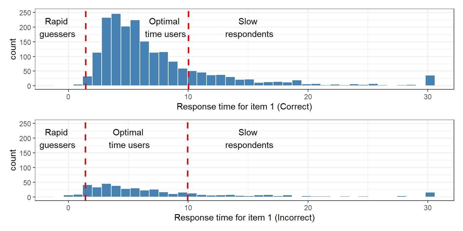
Before we start using the polyscore function, let’s see how rapid guessers, slow respondents, and optimal time users are identified using one of the items (item 1).

library("patchwork")
library("ggplot2")

# Response time distribution for correct
p1 <- ggplot(data = data[data$item_1==1, ], 
             aes(x = rt_1)) +
  geom_histogram(color = "white", 
                 fill = "steelblue", 
                 bins = 40) + ylim(0, 250) + 
  geom_vline(xintercept = median(data[data$item_1==1, "rt_1"])*0.25, 
             linetype="dashed", color = "red", size = 1) +
  geom_vline(xintercept = median(data[data$item_1==1, "rt_1"])*1.75, 
             linetype="dashed", color = "red", size = 1) +
  labs(x = "Response time for item 1 (Correct)") + 
  annotate(geom="text", x = -1, y = 200, label="Rapid\n guessers") + 
  annotate(geom="text", x = 8, y = 200, label="Optimal\n time users") +
  annotate(geom="text", x = 15, y = 200, label="Slow\n respondents") +
  theme_bw()

# Response time distribution for incorrect
p2 <- ggplot(data = data[data$item_1==0, ], 
             aes(x = rt_1)) +
  geom_histogram(color = "white", 
                 fill = "steelblue", 
                 bins = 40) + ylim(0, 250) + 
  geom_vline(xintercept = median(data[data$item_1==0, "rt_1"])*0.25, 
             linetype="dashed", color = "red", size = 1) +
  geom_vline(xintercept = median(data[data$item_1==0, "rt_1"])*1.75, 
             linetype="dashed", color = "red", size = 1) +
  labs(x = "Response time for item 1 (Incorrect)") +
  annotate(geom="text", x = -1, y = 200, label="Rapid\n guessers") + 
  annotate(geom="text", x = 5, y = 200, label="Optimal\n time users") +
  annotate(geom="text", x = 15, y = 200, label="Slow\n respondents") +
  theme_bw()

# Print the plots together
(p1 / p2)

Now we can go ahead and apply polytomous scoring to our data. First, we separate the response and response time portions of the data.

resp_data <- data[, 1:40]
time_data <- data[, 41:80]

Next, we implement the polytomous scoring approach using different combinations of max.score and na.handle. For each combination, we will apply the polyscore function to the items through a loop.

• polydata3_NA: Scores of 0-1-2-3 and not-reached items = NA
• polydata3_IN: Scores of 0-1-2-3 and not-reached items = IN
• polydata4_NA: Scores of 0-1-2-3-4 and not-reached items = NA
• polydata4_IN: Scores of 0-1-2-3-4 and not-reached items = IN

# Define empty matrices to store polytomous responses
polydata3_NA <- matrix(NA, nrow = nrow(resp_data), ncol = ncol(resp_data))
polydata3_IN <- matrix(NA, nrow = nrow(resp_data), ncol = ncol(resp_data))
polydata4_NA <- matrix(NA, nrow = nrow(resp_data), ncol = ncol(resp_data))
polydata4_IN <- matrix(NA, nrow = nrow(resp_data), ncol = ncol(resp_data))

# Run the function within a loop
for(i in 1:ncol(resp_data)) {
  
  polydata3_NA[,i] <- polyscore(resp_data[,i], time_data[,i], max.score = 3, 
                                na.handle = "NA", not.reached = 9, not.answered = 8,  
                                correct = c(0.25, 1.75), incorrect = c(0.25, 1.75))
  
  polydata3_IN[,i] <- polyscore(resp_data[,i], time_data[,i], max.score = 3, 
                                na.handle = "IN", not.reached = 9, not.answered = 8,  
                                correct = c(0.25, 1.75), incorrect = c(0.25, 1.75))
  
  polydata4_NA[,i] <- polyscore(resp_data[,i], time_data[,i], max.score = 4, 
                                na.handle = "NA", not.reached = 9, not.answered = 8,  
                                correct = c(0.25, 1.75), incorrect = c(0.25, 1.75))
  
  polydata4_IN[,i] <- polyscore(resp_data[,i], time_data[,i], max.score = 4, 
                                na.handle = "IN", not.reached = 9, not.answered = 8,  
                                correct = c(0.25, 1.75), incorrect = c(0.25, 1.75))
} 

# Save the data as a data.frame and rename the columns
polydata3_NA <- as.data.frame(polydata3_NA)
names(polydata3_NA) <- names(resp_data)

polydata3_IN <- as.data.frame(polydata3_IN)
names(polydata3_IN) <- names(resp_data)

polydata4_NA <- as.data.frame(polydata4_NA)
names(polydata4_NA) <- names(resp_data)

polydata4_IN <- as.data.frame(polydata4_IN)
names(polydata4_IN) <- names(resp_data)

Let’s quickly see how one of the polytomous data sets looks like after applying polytomous scoring.

head(polydata3_NA)

In this example, we will use polytomously-scored items with Item Response Theory (IRT) to estimate item and person parameters. However, it can also be used with Classical Test Theory (CTT) to calculate raw scores. Regardless of whether IRT or CTT is used, speededness is no longer a nuisance variable because it is used in the operationalization of ability (Tijmstra & Bolsinova, 2018).

Now, we will activate the mirt package (Chalmers, 2012) before conducting IRT analysis.

library("mirt")

Next, we will define a unidimensional model with 40 items and then fit the Graded Response Model (Samejima, 1997) to each polytomous data set.

model <- 'F = 1-40' 

### Apply GRM to each data set
results3_NA <- mirt(data=polydata3_NA, model=model, itemtype="graded", SE=TRUE, verbose=FALSE)
results3_IN <- mirt(data=polydata3_IN, model=model, itemtype="graded", SE=TRUE, verbose=FALSE)
results4_NA <- mirt(data=polydata4_NA, model=model, itemtype="graded", SE=TRUE, verbose=FALSE)
results4_IN <- mirt(data=polydata4_IN, model=model, itemtype="graded", SE=TRUE, verbose=FALSE)

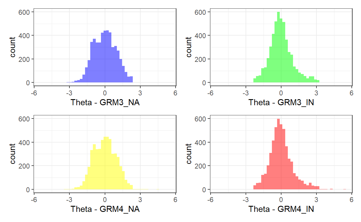
Now, we can see the ability distributions from the four models. The figure shows that the ability distributions become narrower (with high kurtosis) when not-reached items are scored as incorrect, whereas the distribution looks more normal when not-reached items are scored as NA.

# Save theta estimates
theta3_NA <- fscores(results3_NA, method = "EAP")
theta3_IN <- fscores(results3_IN, method = "EAP")
theta4_NA <- fscores(results4_NA, method = "EAP")
theta4_IN <- fscores(results4_IN, method = "EAP")

# Combine theta estimates in a data frame
theta_estimates <- data.frame(
  GRM3_NA = theta3_NA[,1],
  GRM3_IN = theta3_IN[,1],
  GRM4_NA = theta4_NA[,1],
  GRM4_IN = theta4_IN[,1]
)

# Create a histogram for each model
p1 <- ggplot(data = theta_estimates) +
  geom_histogram(aes(x = GRM3_NA), bins = 50, fill = "blue", alpha = 0.5) +
  xlab("Theta - GRM3_NA") + xlim(-5.5, 5.5) + ylim(0, 600) +
  theme_bw()

p2 <- ggplot(data = theta_estimates) +
  geom_histogram(aes(x = GRM3_IN), bins = 50, fill = "green", alpha = 0.5) +
  xlab("Theta - GRM3_IN") + xlim(-5.5, 5.5) + ylim(0, 600) +
  theme_bw()

p3 <- ggplot(data = theta_estimates) +
  geom_histogram(aes(x = GRM4_NA), bins = 50, fill = "yellow", alpha = 0.5) +
  xlab("Theta - GRM4_NA") + xlim(-5.5, 5.5) + ylim(0, 600) +
  theme_bw()

p4 <- ggplot(data = theta_estimates) +
  geom_histogram(aes(x = GRM4_IN), bins = 50, fill = "red", alpha = 0.5) +
  xlab("Theta - GRM4_IN") + xlim(-5.5, 5.5) + ylim(0, 600) +
  theme_bw()

# Combine the histograms
(p1 | p2)/(p3 | p4)

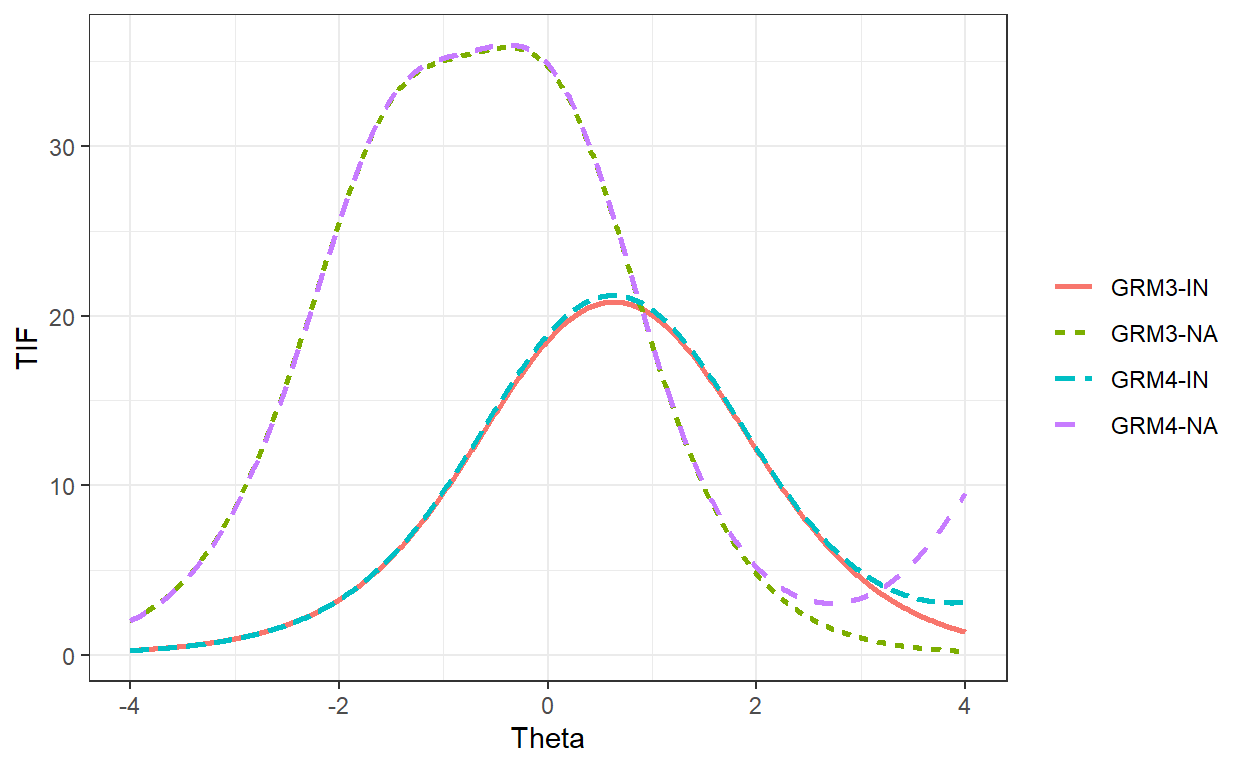
We can also examine test information function (TIF) based on the estimated person parameters using the polytomous scoring approach. The figure shows that GRM3-NA and GRM4-NA are more informative than the other two models where not-reached items were scored as incorrect. Furthermore, compared with GRM3-IN and GRM4-IN, GRM3-NA and GRM4-NA cover a wider range of ability (i.e., theta).

Theta <- matrix(seq(-4, 4, .01))

tif_summary <- data.frame(Theta = Theta,
                          tif = c(testinfo(results3_NA, Theta = Theta),
                                  testinfo(results3_IN, Theta = Theta),
                                  testinfo(results4_NA, Theta = Theta),
                                  testinfo(results4_IN, Theta = Theta)),
                          scoring = c(rep("GRM3-NA", length(Theta)),
                                      rep("GRM3-IN", length(Theta)),
                                      rep("GRM4-NA", length(Theta)),
                                      rep("GRM4-IN", length(Theta))))

ggplot(data = tif_summary, 
       aes(x = Theta, y = tif, linetype = scoring, color = scoring)) +
  geom_line(size = 1) + labs(x = "Theta", y = "TIF") +
  theme_bw() +
  theme(legend.title=element_blank())

Conclusion

Polytomous scoring is an alternative approach when scoring students’ responses in a low-stakes assessment. This approach takes test engagement into account by considering the optimality of response time. Using polytomous scoring can encourage students to avoid response behaviors such as rapid guessing and spending too much time on some items. It should be noted that for this approach to work accurately and effectively, response time cut-off values should be obtained from a large group of students that is representative of the target student population.

---

1. An open-access version of our paper is available:https://journals.sagepub.com/doi/10.1177/0013164421991211.↩︎

2. Smaller percentages can be used for obtaining more conservative cut-off values.↩︎

3. These are items that students view but skip without selecting a valid response option.↩︎