
Introduction
With the COVID-19 pandemic, many educators around the world have begun to use online assessments because students are not able to physically attend classes in order to avoid the spread of the virus. When assessing student learning with online assessments, educators are recommended to avoid long, heavily-weighted exams and instead administer shorter exams more frequently throughout the semester (Kuhfeld et al., 2020). Although this sounds like a good idea in theory, it is easier said than done in practice.
To build shorter exams, educators first need to determine which items should be removed from their existing exams. In addition, they need to ensure that the reliability and other psychometric qualities (e.g., content distribution) of the shortened exams are acceptable. However, making such adjustments manually could be tedious and time-consuming. In this two-part series, I want to demonstrate how to shorten exams (or, any measurement instrument) by automatically selecting the most appropriate items.
In Part I, I will show how to utilize automated test assembly and recursive feature elimination as alternative methods to automatically build shorter versions of educational assessments (e.g., multiple-choice exams, tests, and quizzes).
In Part II, I will demonstrate how to use more advanced algorithms, such as the ant colony optimization (ACO; 🐜) and genetic algorithm (GA; 🧬), for creating short forms of other types of instruments (e.g., psychological scales and surveys).
Let’s get started 💪.
Example
In this example, we will create a hypothetical exam with 80 dichotomously-scored items (i.e., 0 = Incorrect, 1 = Correct). We will assume that the items on the exam are associated with four content domains labeled as ‘A,’ ‘B,’ ‘C,’ and ‘D’ (with 20 items per content domain). We will also assume that a sample of 500 students responded to the items thus far. Because this is a hypothetical exam with no real data, we will need to simulate item responses. The item difficulty distribution will be \(b \sim N(0, 0.7)\) and the ability distribution will be \(\theta \sim N(0, 1)\). We will simulate student responses based on the Rasch model with the xxIRT package (Luo, 2019)1.
library("xxIRT")

# Set the seed so the simulation can be reproduced
set.seed(2021)

# Generate item parameters, abilities, and responses
data <- model_3pl_gendata(
  n_p = 500, # number of students
  n_i = 80, # number of items
  t_dist = c(0, 1), # theta distribution as N(0, 1)
  a = 1, # fix discrimination to 1
  b_dist = c(0, 0.7), # difficulty distribution
  c = 0 # fix guessing to zero (i.e., no guessing)
)

# Save the item parameters as a separate data set
items <- with(data, data.frame(id=paste0("item", 1:80), a=a, b=b, c=c))

# Randomly assign four content domains (A, B, C, or D) to the items
items$content <- sample(LETTERS[1:4], 80, replace=TRUE)
Let’s see the item bank that we have created.
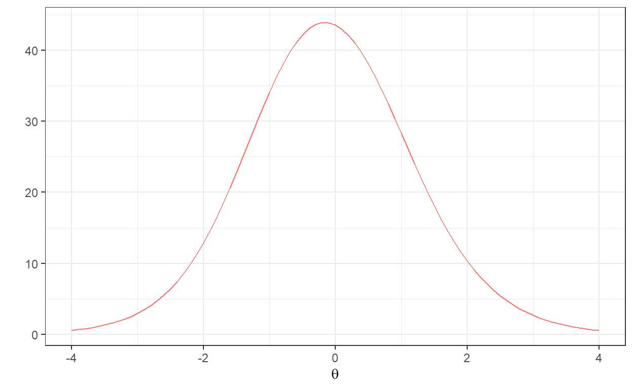
Based on the generated items, we can check out the test information function (TIF) for the entire item bank (i.e., 80 items).
# Test information function
with(data, model_3pl_plot(a, b, c, type="info", total = TRUE))
Finally, we will save the ability parameters and responses as separate data sets.
# Ability
theta <- with(data, data.frame(theta = t))

# Responses
resp <- with(data, as.data.frame(u))
names(resp) <- paste0("item", 1:80)
Automatic Selection of Items
Goal: Assume that using the item bank (i.e., full test with 80 items) generated above, we want to create a short form with only 20 items.
Assumptions: We will assume that: (1) all of the items on the test measure the same latent trait (i.e., the test is unidimensional); (2) the short form will be used for the same student population; and (3) the test does not exhibit any psychometric issues (e.g., mode effect, context effect, or differential item functioning).
Conditions: In the short form, we want to maintain the same content distribution (i.e., an equal number of items from each content domain). Therefore, we will select five items from each content domain (i.e., A, B, C, and D). Furthermore, we want the short form to resemble the full test in terms of reliability and (raw) test scores.
Methodology: With the traditional test assembly approach, we would go through all of the items one by one and pick the appropriate ones based on our judgment. However, this would be highly laborious and inefficient in practice. Therefore, we will use two approaches to automatically select the items:
Automated test assembly as a psychometric approach (IRT parameters are required)2
Recursive feature elimination as a data-driven approach (raw responses are required)
Automated Test Assembly
Automated test assembly (or shortly, ATA) is a mathematical optimization approach that allows us to automatically select items from a large item bank (or, item pool) based on pre-defined psychometric, content, and test administration features3. To solve an ATA task, we can use either a mixed integer programming (MIP) algorithm or a heuristic algorithm. In this example, we will use MIP to look for the optimal test form that meets the psychometric and content requirements (i.e., constraints) that we have identified.
To utilize MIP, we need a solver that will look for the optimal solution based on an objective function (e.g., maximizing test information function) and a set of constraints. In this example, we will use ata_obj_relative to maximize the test information between \(\theta=-0.5\) and \(\theta=0.5\) to mimic the TIF distribution from the full test (i.e, 80 items). In addition, we will use ata_constraint to select five items from each content domain (i.e., A, B, C, and D). For the MIP solver, we will select the open-source solver lp_solve, which is already included in the xxIRT package.
# Define the ATA problem (one form with 20 items)
x <- ata(pool = items, num_form = 1, len = 20, max_use = 1)

# Identify the objective function (maximizing TIF)
x <- ata_obj_relative(x, seq(-0.5, 0.5, .5), 'max')

# Set the content constraints (5 items from each content domain)
x <- ata_constraint(x, 'content', min = 5, max = 5, level = "A")
x <- ata_constraint(x, 'content', min = 5, max = 5, level = "B")
x <- ata_constraint(x, 'content', min = 5, max = 5, level = "C")
x <- ata_constraint(x, 'content', min = 5, max = 5, level = "D")

# Solve the optimization problem
x <- ata_solve(x, 'lpsolve')
optimal solution found, optimum: 9.931 (11.616, 1.685)Once the test assembly is complete, we can see which items have been selected by ATA.
# Selected items
print(x$items)
[[1]]
id a b c content form
3 item3 1 -0.052065 0 C 1
6 item6 1 0.335703 0 D 1
8 item8 1 -0.053997 0 B 1
9 item9 1 0.183544 0 C 1
14 item14 1 0.190379 0 B 1
18 item18 1 -0.439206 0 D 1
19 item19 1 -0.460572 0 B 1
23 item23 1 0.408673 0 B 1
33 item33 1 0.024181 0 C 1
34 item34 1 0.351346 0 A 1
35 item35 1 -0.279468 0 B 1
36 item36 1 0.686681 0 D 1
43 item43 1 -0.371619 0 A 1
46 item46 1 -0.004551 0 D 1
49 item49 1 0.561348 0 D 1
53 item53 1 -0.437516 0 A 1
59 item59 1 -0.416622 0 A 1
68 item68 1 -0.416855 0 A 1
76 item76 1 0.192465 0 C 1
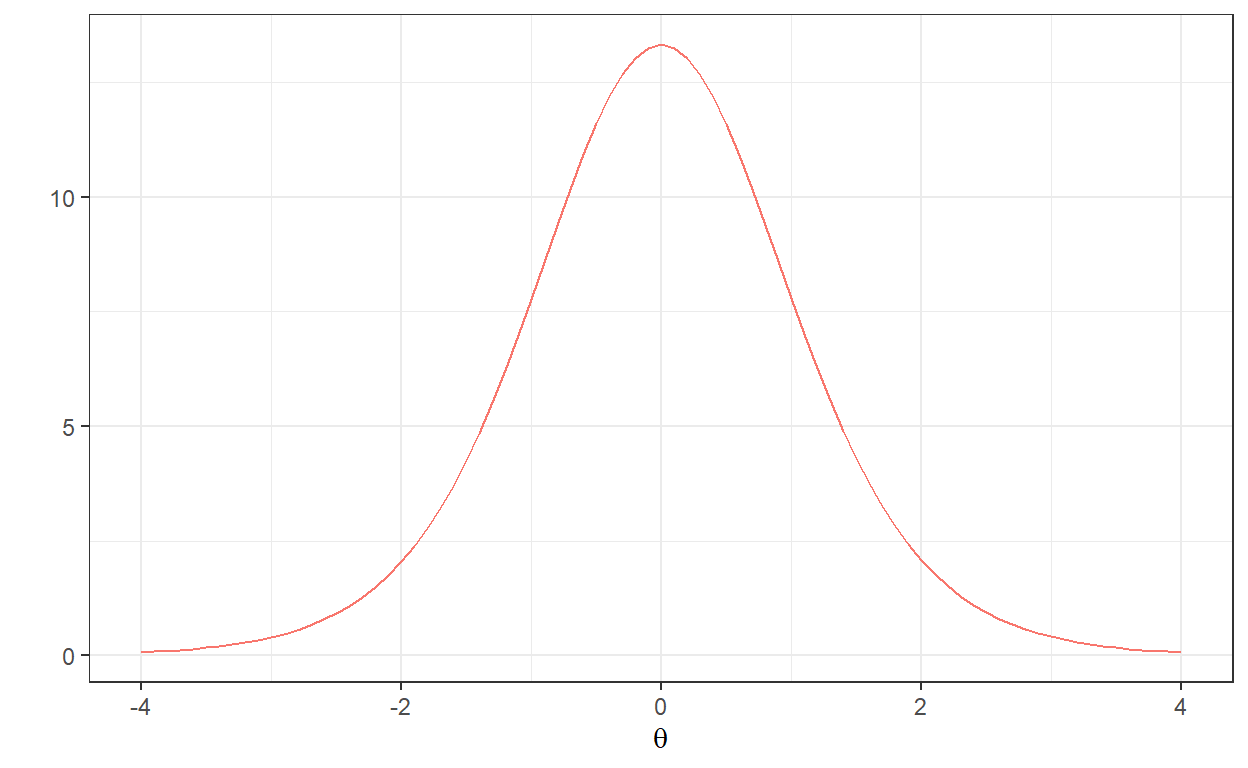
78 item78 1 0.072045 0 C 1In addition, we can draw a plot to see whether the TIF distribution for the short form is similar to the one from the full test.
# TIF for the selected items
with(x$items[[1]],
     model_3pl_plot(a, b, c, type="info", total = TRUE))
Now let’s check the reliability of our new short form as well as the correlation among raw scores (i.e., scores from the whole test vs. scores from the shortened test). We will use the alpha function from the psych package (Revelle, 2019) to compute coefficient alpha for the short form.
 raw_alpha std.alpha G6(smc) average_r   S/N     ase   mean     sd
    0.9133    0.9133  0.9132    0.3449 10.53 0.00562 0.4974 0.3017
 median_r
   0.3481
# Correlation between raw scores
score <- rowSums(resp)
score_ATA <- rowSums(resp[,c(items_ATA)])
cor(score, score_ATA)
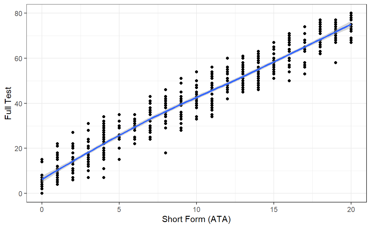
[1] 0.969The reliability of the short form is quite high. Also, there is a very high correlation between the raw scores. Lastly, we will check the scatterplot of the raw scores from the full test (out of 80 points) and the short form (out of 20 points). We will use the ggplot2 package (Wickham, 2016) to create the scatterplot.
library("ggplot2")

# Combine the scores
score1 <- as.data.frame(cbind(score_ATA, score))

# Draw a scatterplot
ggplot(score1, aes(x = score_ATA, y = score)) +
  geom_point() +
  geom_smooth() +
  labs(x = "Short Form (ATA)", y = "Full Test") +
  theme_bw()
Recursive Feature Elimination
The term feature selection may sound unfamiliar to those of us who have studied traditional psychometrics but it is one of the core concepts for data scientists dealing with data mining, predictive modeling, and machine learning.
Feature selection is a process of automatic selection of a subset of relevant features or variables from a set of all features, used in the process of model building. (Dataaspirant)
The primary goal of feature selection is to select the most important predictors by filtering out irrelevant or partially relevant predictors. By selecting the most important predictors, we can build a simple and yet accurate model and avoid problems such as overfitting. There are a number of methods for both supervised and unsupervised feature selection. Feature Engineering and Selection: A Practical Approach for Predictive Models by Kuhn & Johnson (2019) is a great resource for those who want to learn more about feature selection4.
In this example, we will use recursive feature elimination (or shortly, RFE) for automatically selecting items. As a greedy wrapper method, RFE applies backward selection to find the optimal combination of features (i.e., predictors). First, it builds a model based on the entire set of predictors. Then, it removes predictors with the least importance iteratively until a smaller subset of predictors is retained in the model5. In our example, we will use the full set of items (i.e., 80 items) to predict raw scores. RFE will help us eliminate the items that may not be important for the prediction of raw scores6.
To implement RFE for automatic item selection, we will use the randomForest (Liaw & Wiener, 2002) and caret (Kuhn, 2020) packages in R.
The rfe function from caret requires four parameters:
- x: A matrix or data frame of features (i.e., predictors)
- y: The outcome variable to be predicted
- sizes: The number of features that should be retained in the feature selection process
- rfeControl: A list of control options for the feature selection algorithms
Before moving to rfe, we first need to set up the options for rfeControl. The caret package includes a number of functions, such as random forest, naive Bayes, bagged trees, and linear regression7. In this example, we will use the random forest algorithm for model estimation because random forest includes an effective mechanism for measuring feature importance (Kuhn & Johnson, 2019): functions = rfFuncs. In addition, we will add 10-fold cross-validation by using method = “cv” and number = 10.
# Define the control using a random forest selection function
control <- rfeControl(functions = rfFuncs, # random forest
                      method = "cv", # cross-validation
                      number = 10) # the number of folds
Next, we will run the rfe function with the options we have selected above. For this step, we could simply include all of the items together in a single model and select the best 20 items. However, this process may not yield five items from each content domain, which is the content constraint we have specified for our short form. Therefore, we will apply the rfe function to each content domain separately, use sizes = 5 to retain the top five items (i.e., most important items) for each content domain, and then combine the results at the end.
# Run RFE for each content domain within a loop
result <- list()

for(i in c("A", "B", "C", "D")) {
  result[[i]] <- rfe(x = resp[,items[items$content==i,"id"]],
                     y = score,
                     sizes = 5,
                     rfeControl = control)
}

# Extract the results (i.e., first 5 items for each content domain)
items_RFE <- unlist(lapply(result, function(x) predictors(x)[1:5]))
In the following section, we will view the items recommended by RFE and then draw a TIF plot for these items.
# Selected items
print(items[items$id %in% items_RFE, ])
id a b c content
4 item4 1 -0.795227 0 D
6 item6 1 0.335703 0 D
9 item9 1 0.183544 0 C
17 item17 1 -0.641461 0 C
18 item18 1 -0.439206 0 D
19 item19 1 -0.460572 0 B
31 item31 1 -0.106790 0 A
34 item34 1 0.351346 0 A
35 item35 1 -0.279468 0 B
41 item41 1 -0.249472 0 B
42 item42 1 -0.558894 0 C
43 item43 1 -0.371619 0 A
46 item46 1 -0.004551 0 D
53 item53 1 -0.437516 0 A
56 item56 1 -0.499666 0 D
57 item57 1 0.041591 0 C
58 item58 1 -0.551148 0 B
60 item60 1 -0.083425 0 A
72 item72 1 0.529437 0 B
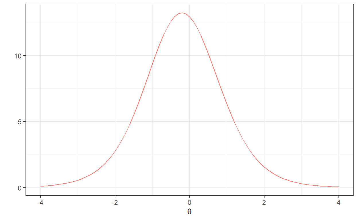
76 item76 1 0.192465 0 C# TIF for the selected items
with(items[items$id %in% items_RFE, ],
model_3pl_plot(a, b, c, type="info", total = TRUE))
Also, we will check the reliability of the short form and correlations between raw scores for the RFE method.
 raw_alpha std.alpha G6(smc) average_r   S/N      ase   mean     sd
    0.9193    0.9193  0.9188    0.3628 11.39 0.005233 0.5495 0.3068
 median_r
0.3659[1] 0.9681As for the ATA method, the correlation between the raw scores is very high for the RFE method. We will also check out the scatterplot of the raw scores.
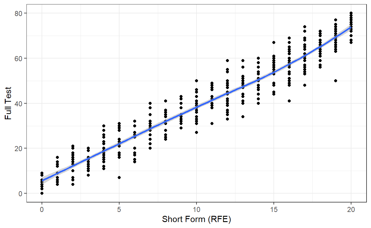
# Combine the scores
score2 <- as.data.frame(cbind(score_RFE, score))

# Draw a scatterplot
ggplot(score2, aes(x = score_RFE, y = score)) +
  geom_point() +
  geom_smooth() +
  labs(x = "Short Form (RFE)", y = "Full Test") +
  theme_bw()
Lastly, we can compute percent-correct scores for the full test and the short forms generated with ATA and RFE to make an overall score comparison. We will use the ggplot2 package to draw a violin plot and check out the score distributions.
# Compute percent-correct scores
score_all <- data.frame(
  test = as.factor(c(rep("Full Test", 500), rep("ATA", 500), rep("RFE", 500))),
  score = c(score/80*100, score_ATA/20*100, score_RFE/20*100)
)

# Make "full test" the first category of the test variable (optional)
score_all$test <- relevel(score_all$test, "Full Test")

# Draw a violin plot (with a boxplot inside)
ggplot(data = score_all, aes(x = test, y = score)) +
  geom_violin(aes(fill = test), trim = FALSE) +
  geom_boxplot(width = 0.2)+
  scale_fill_manual(values = c("#00AFBB", "#E7B800", "#FC4E07")) +
  labs(x = "", y = "Percent-Correct Scores") +
  theme_bw() + theme(legend.position="none")
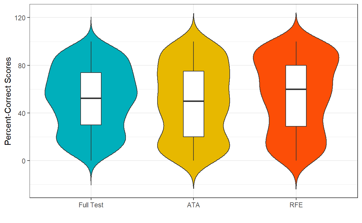
The violin plot shows that the score distributions are not exactly the same but they are pretty similar.
Conclusion
Both methods (i.e., ATA and RFE) appear to yield very similar (and very good!) results in terms of reliability and correlations between raw scores, although they recommended different sets of items for the short form. This may not be a surprising finding because we generated a nice and clean data set (e.g., no missing responses, no outliers, etc.) based on a psychometric model (i.e., Rasch). Automatic item selection with ATA and RFE may produce less desirable results if:
- the sample size is smaller,
- non-random missingness is present in the response data set, and
- there are problematic items (e.g., items with low discrimination or high guessing).
The model_3pl_estimate_mmle function in the same package can be used to estimate item parameters based on raw response data.↩︎
Item response theory (IRT) is a psychometric framework for the design, analysis, and scoring of tests, questionnaires, and similar instruments. If you are not familiar with IRT, you can move to the second approach: Recursive feature elimination.↩︎
You can check out Van der Linden (2006)’s “Linear Models for Optimal Test Design” for further information on ATA.↩︎
Max Kuhn is also the author of the famous
caretpackage.↩︎See http://www.feat.engineering/recursive-feature-elimination.html for more information on RFE↩︎
This could also be used for predicting person ability estimates in IRT or another external criterion.↩︎
See https://topepo.github.io/caret/recursive-feature-elimination.html for further information.↩︎