Explanatory IRT Models in R

Explanatory item response modeling (EIRM) is a flexible framework that allows researchers to model both person and item characteristics as predictors together. In this post, I demonstrate how to use the eirm package to estimate explanatory IRT models in R.

(4 min read)

Introduction

Explanatory item response modeling (shortly EIRM) was first proposed by De Boeck & Wilson (2004) as an alternative to traditional item response model. This framework allows us to turn traditional item response theory (IRT) models into explanatory models with additional predictors. Explanatory IRT models aim to explain how item properties (e.g., content, cognitive complexity, and presence of visual elements) and person characteristics (e.g., gender, race, and English language learner (ELL) status) affect the persons’ responses to items. For a brief introduction to EIRM, you can check out Wilson, De Boeck, and Carstensen’s chapter here.

In De Boeck & Wilson (2004)’s book, the authors describe how to estimate explanatory IRT models using the SAS statistical software program. Given the growing popularity of R in the psychometric/measurement community, De Boeck et al. (2011) published a nice article that describes how to estimate the same models using the lme4 package (Bates et al., 2015) in R. Since then, I have been using the lme4 package to estimate explanatory IRT models for my research projects. For example, we evaluated measurement invariance of two developmental assets, Support and Positive Identity, across grade levels and ELL subgroups of Latino students in 6th through 12th grade (Bulut et al., 2015). Also, we investigated whether the linguistic complexity of items leads to gender differential item functioning (DIF) in mathematics assessments (Kan & Bulut, 2014).

One problem that we often had to deal with when using lme4 was the format of item responses. The lme4 package assumes a binomial distribution for item responses, which means responses must be dichotomous (i.e., 0 and 1). Although this is not a problem for dichotomous data based on multiple-choice items, it is a major drawback for polytomous data based on rating scale items (e.g., Likert scales). Therefore, we had to develop a new way to transform polytomous responses into dichotomous responses without losing the original response structure (Stanke & Bulut, 2019). Recently, I decided to share this method in a new package that would faciliate the estimation of explanatory IRT models for both dichotomous and polytomous response data. Therefore, I created the eirm package (Bulut, 2021), which is essentially a wrapper for the lme4 package (Bates et al., 2015). The eirm function in the package allows users to define an explanatory IRT model based on item-level and person-level predictors.

Example

In this post, I will show how to use the eirm package to estimate explanatory IRT models with polytomous response data. For more examples, you can check out the eirm website: https://okanbulut.github.io/eirm/. The eirm package is currently available on CRAN. It can be downloaded and installed using install.packages(“eirm”).

I will use the verbal aggression dataset in the lme4 package to demonstrate the estimation process. The dataset includes responses to a questionnaire on verbal aggression and additional variables related to items and persons. A preview of the data set is shown below:

library("eirm")

data("VerbAgg")

head(VerbAgg)

  Anger Gender        item    resp id btype  situ mode r2
1    20      M S1WantCurse      no  1 curse other want  N
2    11      M S1WantCurse      no  2 curse other want  N
3    17      F S1WantCurse perhaps  3 curse other want  Y
4    21      F S1WantCurse perhaps  4 curse other want  Y
5    17      F S1WantCurse perhaps  5 curse other want  Y
6    21      F S1WantCurse     yes  6 curse other want  Y

In the dataset, the variable resp represents each person’s response to the items on the questionnaire. There are three values for resp: yes, perhaps, and no. Therefore, we need to transform these poytomous responses into dichotomous responses. To reformat the data, we will use the polyreformat function in the eirm package. The following example demonstrates how polytomous responses in the verbal aggression dataset can be reformatted into a dichotomous form:

VerbAgg2 <- polyreformat(data=VerbAgg, id.var = "id", var.name = "item", val.name = "resp")

head(VerbAgg2)

  Anger Gender        item    resp id btype  situ mode r2
1    20      M S1WantCurse      no  1 curse other want  N
2    11      M S1WantCurse      no  2 curse other want  N
3    17      F S1WantCurse perhaps  3 curse other want  Y
4    21      F S1WantCurse perhaps  4 curse other want  Y
5    17      F S1WantCurse perhaps  5 curse other want  Y
6    21      F S1WantCurse     yes  6 curse other want  Y
  polycategory polyresponse                polyitem
1  cat_perhaps            0 S1WantCurse.cat_perhaps
2  cat_perhaps            0 S1WantCurse.cat_perhaps
3  cat_perhaps            1 S1WantCurse.cat_perhaps
4  cat_perhaps            1 S1WantCurse.cat_perhaps
5  cat_perhaps            1 S1WantCurse.cat_perhaps
6  cat_perhaps           NA S1WantCurse.cat_perhaps

In the reformatted data, polyresponse is the new response variable (i.e., pseudo-dichotomous version of the original response variable resp) and polycategory represents the response categories. Based on the reformatted data, each item has two rows based on the following rules:

• If polycategory = “cat_perhaps” and resp = “no,” then polyresponse = 0
• If polycategory = “cat_perhaps” and resp = “perhaps,” then polyresponse = 1
• If polycategory = “cat_perhaps” and resp = “yes,” then polyresponse = NA

and

• If polycategory = “cat_yes” and resp = “no,” then polyresponse = NA
• If polycategory = “cat_yes” and resp = “perhaps,” then polyresponse = 0
• If polycategory = “cat_yes” and resp = “yes,” then polyresponse = 1

Now we can estimate an explanatory IRT model using the reformatted data. The following model explains only the first threshold (i.e., threshold from no to perhaps) based on three predictors:

mod1 <- eirm(formula = "polyresponse ~ -1 + situ + btype + mode + (1|id)", 
             data = VerbAgg2)

The regression-like formula polyresponse ~ -1 + situ + btype + mode + (1|id) describes the dependent variable (polyresponse) and predictors (situ, btype, and mode). Also, (1|id) refers to the random effects for persons represented by the id column in the data set. Using the print function or simply typing mod1 in the R console, we can print out the estimated coefficients for the predictors:

print(mod1)

EIRM formula: "polyresponse ~ -1 + situ + btype + mode + (1|id)" 

Number of persons: 316 

Number of observations: 9665 

Number of predictors: 5 

Parameter Estimates:

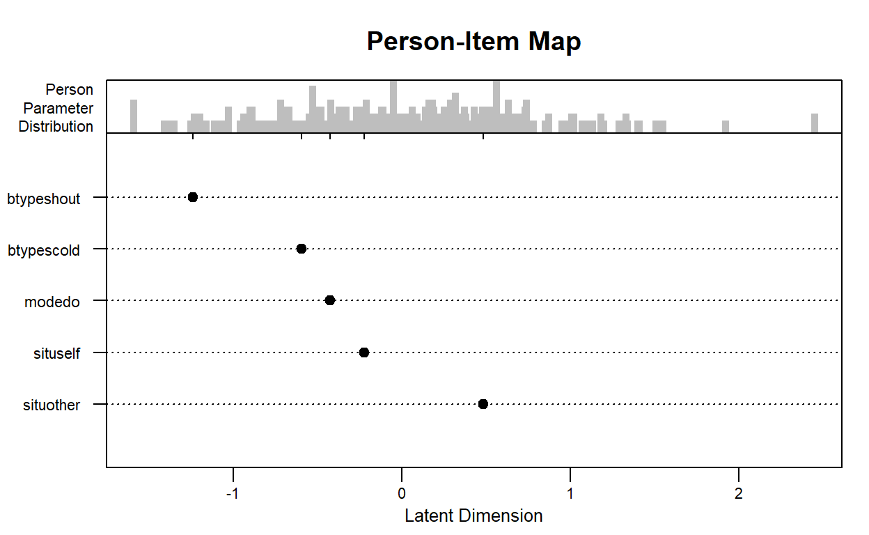
           Easiness    S.E. z-value    p-value
situother    0.4846 0.06628   7.312  2.626e-13
situself    -0.2239 0.06548  -3.419  6.277e-04
btypescold  -0.5936 0.05334 -11.128  9.208e-29
btypeshout  -1.2387 0.05810 -21.319 7.562e-101
modedo      -0.4264 0.04576  -9.319  1.179e-20

Note: The estimated parameters above represent 'easiness'.
Use difficulty = TRUE to get difficulty parameters.

The mod1 object is essentially a glmerMod-class object from the lme4 package (Bates et al., 2015). All glmerMod results for the estimated model can seen with mod1$model. For example, estimated random effects for persons (i.e., theta estimates) can be obtained using:

theta <- ranef(mod1$model)$id
head(theta)

It is possible to visualize the parameters using an item-person map. Note that this plot is a modified version of the plotPImap function from the eRm package (Mair et al., 2020). Aesthetic elements such as axis labels and plot title can be added to the plot. Please run ?plot.eirm for further details on the plot option.

plot(mod1)

The previous model could be modified to explain the first threshold (i.e., threshold from no to perhaps) and second threshold (perhaps to yes) based on explanatory variables using the following codes:

mod2 <- eirm(formula = "polyresponse ~ -1 + btype + situ + mode + 
             polycategory + polycategory:btype + (1|id)", data = VerbAgg2)

Conclusion

Before I conclude this post, I want to mention a few caveats with the eirm package. First, the eirm package is using a different optimizer to speed up the estimation process. However, as the size of response data (i.e., items and persons) increases, the estimation duration may increase significantly. Second, it is possible to use dichotomous and polytomous items within the same model. In that case, a single difficulty is estimated for dichotomous items (i.e., Rasch model) and multiple thresholds for polytomous items (i.e., either Partial Credit model or Rating Scale model). Lastly, the eirm package is not capable of estimating a discrimination parameter for the items (just like lme4 can’t). Structural equation modeling could be a good alternative for those who want to estimate both discrimination and difficulty parameters for the items.